手把手教 | 深度學習庫PyTorch（附程式碼）

介紹

每隔一段時間，就會有一個有潛力改變深度學習格局的python庫誕生，PyTorch就是其中一員。

在過去的幾周裡，我一直沉浸在PyTorch中，我被它的易用性所吸引。在我使用過的各種深度學習庫中，到目前為止PyTorch是最靈活最易用的。

在本文中，我們將以一種更實用的方式探索PyTorch, 其中包含了基礎知識和案例研究。同時我們還將對比分別用numpy和PyTorch從頭構建的神經網路，以檢視它們在具體實現中的相似之處。

讓我們開始吧！

註意：本文假定你對深度學習有基本的認知。如果想快速瞭解，請先閱讀此文https://www.analyticsvidhya.com/blog/2016/03/introduction-deep-learning-fundamentals-neural-networks/

目錄

• PyTorch概覽

• 深入技術

• 構建神經網路之Numpy VS. PyTorch

• 與其他深度學習庫對比

• 案例研究 — 用PyTorch解決影象識別問題

PyTorch概覽

PyTorch的創作者說他們遵從指令式(imperative)的程式設計哲學。這就意味著我們可以立即執行計算。這一點正好符合Python的程式設計方法學，因為我們沒必要等到程式碼全部寫完才知道它是否能執行。我們可以輕鬆地執行一部分程式碼並實時檢查它。對於我這樣的神經網路除錯人員而言，這真是一件幸事。

PyTorch是一個基於python的庫，它旨在提供一個靈活的深度學習開發平臺。

PyTorch的工作流程盡可能接近Python的科學計算庫— numpy。

你可能會問，我們為什麼要用PyTorch來構建深度學習模型呢？我列舉三點來回答這個問題：

• 易用的API：像Python一樣簡單易用；

• 支援Python：如上所說，PyTorch平滑地與Python資料科學棧整合。它與Numpy如此相似，你甚至都不會註意到其中的差異；

• 動態計算圖：PyTorch沒有提供具有特定功能的預定義圖，而是提供給我們一個框架用於構建計算圖，我們甚至可以在執行時更改它們。這對於一些情況是很有用的，比如我們在建立一個神經網路時事先並不清楚需要多少記憶體。

使用PyTorch還有其他一些好處，比如它支援多GPU，自定義資料載入器和簡化的前處理器。

自從2016年1月初釋出以來，許多研究人員已經將它納入自己的工具箱，因為它易於構建新穎甚至非常複雜的圖。話雖如此，PyTorch要想被大多數資料科學從業者所接受還需時日，因為它既是新生事物而且還在”建設中”。

深入技術

在深入細節之前，我們先瞭解一下PyTorch的工作流程。

PyTorch使用了指令式程式設計正規化。也就是說，用於構建圖所需的每行程式碼都定義了該圖的一個元件。即使在圖被完全構建好之前，我們也可以在這些元件上獨立地執行計算。這被稱為 ”define-by-run” 方法。

Source: http://pytorch.org/about/

安裝PyTorch非常簡單。你可以根據你的系統，按照官方檔案中提到的步驟操作。例如，下麵是基於我的選項所用的命令：

conda install pytorch torchvision cuda91 -cpytorch

在我們開始使用PyTorch時，應該瞭解的主要元素是：

• PyTorch張量(Tensors)

• 數學運算

• Autograd模組

• Optim模組

• nn模組

下麵，我們將詳細介紹每一部分。

1. PyTorch張量

張量就是多維陣列。PyTorch中的張量與Numpy中的ndarrays很相似，除此之外，PyTorch中的張量還可以在GPU上使用。PyTorch支援各種型別的張量。

你可以定義一個簡單的一維矩陣如下：

# import pytorch

import torch

# define a tensor

torch.FloatTensor([2])

2

[torch.FloatTensor of size 1]

2. 數學運算

與numpy一樣，科學計算庫有效地實現數學函式是非常重要的。PyTorch提供了一個類似的介面，你可以使用超過200多種數學運算。

以下是一個簡單的加法操作例子：

a = torch.FloatTensor([2])

b = torch.FloatTensor([3])

a + b

5

[torch.FloatTensor of size 1]

這難道不像是一個典型的python方法嗎？我們也可以在定義過的PyTorch張量上執行各種矩陣運算。例如，我們轉置一個二維矩陣：

matrix = torch.randn(3, 3)

matrix

-1.3531 -0.5394  0.8934

 1.7457 -0.6291 -0.0484

-1.3502 -0.6439 -1.5652

[torch.FloatTensor of size 3x3]

matrix.t()

-1.3531  1.7457  -1.3502

-0.5394 -0.6291  -0.6439

 0.8934  -0.0484  -1.5652

[torch.FloatTensor of size 3x3]

3. Autograd模組

PyTorch使用了一種被稱為自動微分(automaticdifferentiation)的技術。也就是說，我們有一個記錄器，記錄了我們已經執行的操作，然後它向後重播以計算我們的梯度。這種技術在構建神經網路時特別有用，因為我們在前向傳播時計算引數的微分，這可以減少每一個epoch的計算時間。

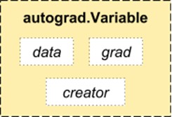
Source: http://pytorch.org/about/

from torch.autograd import Variable

x = Variable(train_x)

y = Variable(train_y, requires_grad=False)

4. Optim模組

Torch.optim是一個模組，它實現了用於構建神經網路的各種最佳化演演算法。大多數常用的方法已被支援，所以我們無需從頭開始構建他們（除非你想！）。

以下是使用Adam最佳化器的一段程式碼：

optimizer = torch.optim.Adam(model.parameters(), lr=learning_rate)

5. nn模組

PyTorch的autograd可以很容易的定義計算圖並且求梯度，但是原始的autograd對於定義複雜的神經網路可能有點過於低階。這也是nn模組可以幫忙的地方。

Nn包定義了一組模組，我們可以將其視為一個神經網路層，它可以從輸入產生輸出，並且可能有一些可訓練的權重。

你可以把nn模組當做是PyTorch的keras!

import torch

# define model

model = torch.nn.Sequential(

 torch.nn.Linear(input_num_units, hidden_num_units),

 torch.nn.ReLU(),

 torch.nn.Linear(hidden_num_units, output_num_units),

)

loss_fn = torch.nn.CrossEntropyLoss()

現在你知道了PyTorch的基本元件，你可以輕鬆地從頭構建自己的神經網路。如果你想知道具體怎麼做，繼續往下讀。

構建神經網路之 Numpy VS. PyTorch

之前我提到PyTorch和Numpy非常相似，讓我們看看為什麼。在本節中，我們會看到一個簡單的用於解決二元分類問題的神經網路如何實現。你可以透過https://www.analyticsvidhya.com/blog/2017/05/neural-network-from-scratch-in-python-and-r/獲得深入的解釋。

## Neural network in numpy

import numpy as np

#Input array

X=np.array([[1,0,1,0],[1,0,1,1],[0,1,0,1]])

#Output

y=np.array([[1],[1],[0]])

#Sigmoid Function

def sigmoid (x):

 return 1/(1 + np.exp(-x))

#Derivative of Sigmoid Function

def derivatives_sigmoid(x):

 return x * (1 - x)

#Variable initialization

epoch=5000 #Setting training iterations

lr=0.1 #Setting learning rate

inputlayer_neurons = X.shape[1] #number of features in data set

hiddenlayer_neurons = 3 #number of hidden layers neurons

output_neurons = 1 #number of neurons at output layer

#weight and bias initialization

wh=np.random.uniform(size=(inputlayer_neurons,hiddenlayer_neurons))

bh=np.random.uniform(size=(1,hiddenlayer_neurons))

wout=np.random.uniform(size=(hiddenlayer_neurons,output_neurons))

bout=np.random.uniform(size=(1,output_neurons))

for i in range(epoch):

  #Forward Propogation

  hidden_layer_input1=np.dot(X,wh)

  hidden_layer_input=hidden_layer_input1 + bh

  hiddenlayer_activations = sigmoid(hidden_layer_input)

  output_layer_input1=np.dot(hiddenlayer_activations,wout)

  output_layer_input= output_layer_input1+ bout

  output = sigmoid(output_layer_input)

  #Backpropagation

  E = y-output

  slope_output_layer = derivatives_sigmoid(output)

  slope_hidden_layer = derivatives_sigmoid(hiddenlayer_activations)

  d_output = E * slope_output_layer

  Error_at_hidden_layer = d_output.dot(wout.T)

  d_hiddenlayer = Error_at_hidden_layer * slope_hidden_layer

  wout += hiddenlayer_activations.T.dot(d_output) *lr

  bout += np.sum(d_output, axis=0,keepdims=True) *lr

  wh += X.T.dot(d_hiddenlayer) *lr

  bh += np.sum(d_hiddenlayer, axis=0,keepdims=True) *lr

print('actual :\n', y, '\n')

print('predicted :\n', output)

現在，嘗試發現PyTorch超級簡單的實現與之前的差異（下麵程式碼中差異部分用粗體字表示）。

## neural network in pytorch

import torch

#Input array

X = torch.Tensor([[1,0,1,0],[1,0,1,1],[0,1,0,1]])

#Output

y = torch.Tensor([[1],[1],[0]])

#Sigmoid Function

def sigmoid (x):

  return 1/(1 + torch.exp(-x))

#Derivative of Sigmoid Function

def derivatives_sigmoid(x):

  return x * (1 - x)

#Variable initialization

epoch=5000 #Setting training iterations

lr=0.1 #Setting learning rate

inputlayer_neurons = X.shape[1] #number of features in data set

hiddenlayer_neurons = 3 #number of hidden layers neurons

output_neurons = 1 #number of neurons at output layer

#weight and bias initialization

wh=torch.randn(inputlayer_neurons, hiddenlayer_neurons).type(torch.FloatTensor)

bh=torch.randn(1, hiddenlayer_neurons).type(torch.FloatTensor)

wout=torch.randn(hiddenlayer_neurons, output_neurons)

bout=torch.randn(1, output_neurons)

for i in range(epoch):

  #Forward Propogation

  hidden_layer_input1 = torch.mm(X, wh)

  hidden_layer_input = hidden_layer_input1 + bh

  hidden_layer_activations = sigmoid(hidden_layer_input)

  output_layer_input1 = torch.mm(hidden_layer_activations, wout)
  output_layer_input = output_layer_input1 + bout
  output = sigmoid(output_layer_input1)
 
  #Backpropagation
  E = y-output
  slope_output_layer = derivatives_sigmoid(output)
  slope_hidden_layer = derivatives_sigmoid(hidden_layer_activations)
  d_output = E * slope_output_layer
  Error_at_hidden_layer = torch.mm(d_output, wout.t())
  d_hiddenlayer = Error_at_hidden_layer * slope_hidden_layer
  wout += torch.mm(hidden_layer_activations.t(), d_output) *lr
  bout += d_output.sum() *lr
  wh += torch.mm(X.t(), d_hiddenlayer) *lr
  bh += d_output.sum() *lr
print('actual :\n', y, '\n')
print('predicted :\n', output)
 


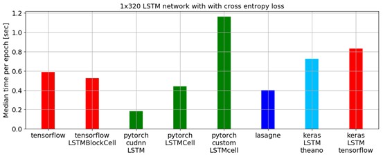
與其他深度學習庫對比




在一個基準測試指令碼中，透過比較最低的epoch中位數時間，PyTorch在訓練一個Long Short Term Memory(LSTM)網路方面勝過了所有其他主要的深度學習庫，參加下圖：
 



用於資料載入的APIs在PyTorch中設計良好。介面在資料集，取樣器和資料載入器中指定。
 
在比較TensorFlow中的資料載入工具(readers, queues等等)時，我發現PyTorch的資料載入模組非常易於使用。另外，PyTorch在我們嘗試構建神經網路時是無縫銜接的，所以我們不必像keras那樣依賴第三方高階庫（keras依賴tensorflow或theano）。
 
另一方面，我不推薦使用PyTorch進行部署。 PyTorch尚處於發展中。正如PyTorch開發人員所說：“我們看到的是使用者首先建立一個PyTorch模型，當他們準備將模型部署到生產環境時，他們只需將其轉換成Caffe 2模型，然後將其釋出到移動平臺或其他平臺。“


案例研究：用PyTorch解決影象識別問題


為了熟悉PyTorch，我們將解決Analytics Vidhya的深度學習實踐問題 - 識別數字。我們來看看我們的問題陳述：
 
我們的問題是一個影象識別問題，從一個給定的28×28畫素的影象中識別數字。我們有一部分影象用於訓練，其餘部分用於測試我們的模型。
 
首先，下載訓練和測試檔案。該資料集包含所有影象的壓縮檔案，並且train.csv和test.csv都具有相應訓練和測試影象的名稱。資料集中不提供任何其他特徵，只是以'.png'格式提供原始影象。
 
讓我們開始吧：
 
步驟0：準備


1. 匯入所有必要的庫：


# import modules
%pylab inline
import os
import numpy as np
import pandas as pd
from scipy.misc import imread
from sklearn.metrics import accuracy_score
 
2. 設定種子值，以便我們可以控制模型的隨機性


# To stop potential randomness
seed = 128
rng = np.random.RandomState(seed)


3. 第一步是設定目錄路徑，以便安全儲存！


root_dir = os.path.abspath('.')
data_dir = os.path.join(root_dir, 'data')
 
# check for existence
os.path.exists(root_dir), os.path.exists(data_dir)
 
步驟1：資料載入和預處理


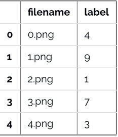
1. 現在我們來讀取資料集。他們是.csv格式，並且具有相應標簽的檔案名。
 
# load dataset
train = pd.read_csv(os.path.join(data_dir, 'Train', 'train.csv'))
test = pd.read_csv(os.path.join(data_dir, 'Test.csv'))
 
sample_submission = pd.read_csv(os.path.join(data_dir, 'Sample_Submission.csv'))
 
train.head()



 
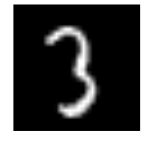
2. 我們看一下資料是什麼樣子，讀取圖片並顯示。


# print an image
img_name = rng.choice(train.filename)
filepath = os.path.join(data_dir, 'Train', 'Images', 'train', img_name)
 
img = imread(filepath, flatten=True)
 
pylab.imshow(img, cmap='gray')
pylab.axis('off')
pylab.show()

3. 為了便於資料操作，我們將所有圖片儲存為numpy陣列。
 
# load images to create train and test set
temp = []
for img_name in train.filename:
  image_path = os.path.join(data_dir, 'Train', 'Images', 'train', img_name)
  img = imread(image_path, flatten=True)
  img = img.astype('float32')
  temp.append(img)
train_x = np.stack(temp)
 
train_x /= 255.0
train_x = train_x.reshape(-1, 784).astype('float32')
 
temp = []
for img_name in test.filename:
  image_path = os.path.join(data_dir, 'Train', 'Images', 'test', img_name)
  img = imread(image_path, flatten=True)
  img = img.astype('float32')
  temp.append(img)
test_x = np.stack(temp)
 
test_x /= 255.0
test_x = test_x.reshape(-1, 784).astype('float32')
 
train_y = train.label.values
 
4. 由於這是一個典型的ML問題，為了測試我們模型的正確功能，我們建立了一個驗證集(validation set)。我們以70:30的比例來劃分訓練集和驗證集。
 
# create validation set
split_size = int(train_x.shape[0]*0.7)
 
train_x, val_x = train_x[:split_size], train_x[split_size:]
train_y, val_y = train_y[:split_size], train_y[split_size:]
 
步驟2：構建模型


5. 現在來到了主要部分，即定義我們的神經網路架構。我們定義了一個3層神經網路即輸入，隱藏和輸出層。輸入和輸出層中的神經元數量是固定的，因為輸入是我們的28×28影象，並且輸出是代表類別的10×1向量。我們在隱藏層中使用50個神經元。在這裡，我們使用Adam作為最佳化演演算法，它是梯度下降演演算法的有效變種。
 
import torch
from torch.autograd import Variable
# number of neurons in each layer
input_num_units = 28*28
hidden_num_units = 500
output_num_units = 10
 
# set remaining variables
epochs = 5
batch_size = 128
learning_rate = 0.001


6. 訓練模型的時間到了
 
# define model
model = torch.nn.Sequential(
  torch.nn.Linear(input_num_units, hidden_num_units),
  torch.nn.ReLU(),
  torch.nn.Linear(hidden_num_units, output_num_units),
)
loss_fn = torch.nn.CrossEntropyLoss()
 
# define optimization algorithm
optimizer = torch.optim.Adam(model.parameters(), lr=learning_rate)
## helper functions
# preprocess a batch of dataset
def preproc(unclean_batch_x):
  """Convert values to range 0-1"""
  temp_batch = unclean_batch_x / unclean_batch_x.max()
  return temp_batch
 
# create a batch
def batch_creator(batch_size):
  dataset_name = 'train'
  dataset_length = train_x.shape[0]
  
  batch_mask = rng.choice(dataset_length, batch_size)
  
  batch_x = eval(dataset_name + '_x')[batch_mask]
  batch_x = preproc(batch_x)
  
  if dataset_name == 'train':
    batch_y = eval(dataset_name).ix[batch_mask, 'label'].values
  
  return batch_x, batch_y
# train network
total_batch = int(train.shape[0]/batch_size)
 
for epoch in range(epochs):
  avg_cost = 0
  for i in range(total_batch):
    # create batch
    batch_x, batch_y = batch_creator(batch_size)
 
    # pass that batch for training
    x, y = Variable(torch.from_numpy(batch_x)), Variable(torch.from_numpy(batch_y), requires_grad=False)
    pred = model(x)
 
    # get loss
    loss = loss_fn(pred, y)
 
    # perform backpropagation
    loss.backward()
    optimizer.step()
    avg_cost += loss.data[0]/total_batch
 
  print(epoch, avg_cost)
# get training accuracy
x, y = Variable(torch.from_numpy(preproc(train_x))), Variable(torch.from_numpy(train_y), requires_grad=False)
pred = model(x)
 
final_pred = np.argmax(pred.data.numpy(), axis=1)
 
accuracy_score(train_y, final_pred)
# get validation accuracy
x, y = Variable(torch.from_numpy(preproc(val_x))), Variable(torch.from_numpy(val_y), requires_grad=False)
pred = model(x)
final_pred = np.argmax(pred.data.numpy(), axis=1)
 
accuracy_score(val_y, final_pred)


訓練得分是：


0.8779008746355685


而驗證得分是：


0.867482993197279


這是一個很令人印象深刻的分數，尤其是我們只是在5個epochs上訓練了一個非常簡單的神經網路。


結語


我希望這篇文章能讓你看到PyTorch如何改變構建深度學習模型的觀點。在這篇文章中，我們只是淺嘗輒止。為了深入研究，你可以閱讀PyTorch官方頁面上的檔案和教程。


在接下來的幾篇文章中，我將使用PyTorch進行音訊分析，並且我們將嘗試構建語音處理的深度學習模型。敬請關註！


你用過PyTorch構建應用程式或者將其用在任何資料科學專案裡嗎？請在下麵的評論中告訴我。


原文連結：https://www.analyticsvidhya.com/blog/2018/02/pytorch-tutorial/




譯者簡介：和中華，留德軟體工程碩士。由於對機器學習感興趣，碩士論文選擇了利用遺傳演演算法思想改進傳統kmeans。目前在杭州進行大資料相關實踐。加入資料派THU希望為IT同行們盡自己一份綿薄之力，也希望結交許多志趣相投的小夥伴。
本文轉自：資料派THU 公眾號；

END

關聯閱讀：




原創系列文章：
1：從0開始搭建自己的資料運營指標體系（概括篇）
2 ：從0開始搭建自己的資料運營指標體系（定位篇）

3 ：從0開始搭建自己的資料運營體系（業務理解篇）
4 ：資料指標的構建流程與邏輯

5 ：系列 ：從資料指標到資料運營指標體系
6:   實戰 ：為自己的公號搭建一個資料運營指標體系
7:  從0開始搭建自己的資料運營指標體系（運營活動分析）
資料運營 關聯文章閱讀：  
運營入門，從0到1搭建資料分析知識體系    
推薦 ：資料分析師與運營協作的9個好習慣

乾貨 ：手把手教你搭建資料化使用者運營體系
推薦 ：最用心的運營資料指標解讀
乾貨 : 如何構建資料運營指標體系
從零開始，構建資料化運營體系
乾貨 ：解讀產品、運營和資料三個基友關係

乾貨 ：從0到1搭建資料運營體系
資料分析、資料產品 關聯文章閱讀：
乾貨 ：資料分析團隊的搭建和思考

關於使用者畫像那些事，看這一文章就夠了

資料分析師必需具備的10種分析思維。

如何構建大資料層級體系，看這一文章就夠了

乾貨 ： 聚焦於使用者行為分析的資料產品

如何構建大資料層級體系，看這一文章就夠了

80%的運營註定了打雜？因為你沒有搭建出一套有效的使用者運營體系
從底層到應用，那些資料人的必備技能

讀懂使用者運營體系：使用者分層和分群
做運營必須掌握的資料分析思維，你還敢說不會做資料分析












贊賞



長按二維碼向我轉賬


受蘋果公司新規定影響，微信 iOS 版的贊賞功能被關閉，可透過二維碼轉賬支援公眾號。


閱讀原文





即將開啟""小程式

取消

開啟