小姐姐帶你一起學：如何用Python實現7種機器學習演演算法（附程式碼）-知識星球

導讀：Python 被稱為是最接近 AI 的語言。最近一位名叫Anna-Lena Popkes的小姐姐在GitHub上分享了自己如何使用Python（3.6及以上版本）實現7種機器學習演演算法的筆記，並附有完整程式碼。

所有這些演演算法的實現都沒有使用其他機器學習庫。這份筆記可以幫大家對演演算法以及其底層結構有個基本的瞭解，但並不是提供最有效的實現。

小姐姐她是德國波恩大學電腦科學專業的研究生，主要關註機器學習和神經網路。

七種演演算法包括：

線性回歸演演算法
Logistic 回歸演演算法
感知器
K 最近鄰演演算法
K 均值聚類演演算法
含單隱層的神經網路
多項式的 Logistic 回歸演演算法

01 線性回歸演演算法

線上性回歸中，我們想要建立一個模型，來擬合一個因變數 y 與一個或多個獨立自變數(預測變數) x 之間的關係。

給定：

資料集
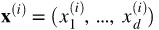
是d-維向量

是一個標的變數，它是一個標量

線性回歸模型可以理解為一個非常簡單的神經網路：

它有一個實值加權向量
它有一個實值偏置量 b
它使用恆等函式作為其啟用函式

線性回歸模型可以使用以下方法進行訓練

a) 梯度下降法

b) 正態方程(封閉形式解)：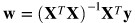

其中 X 是一個矩陣，其形式為，包含所有訓練樣本的維度資訊。

而正態方程需要計算的轉置。這個操作的計算複雜度介於）和之間，而這取決於所選擇的實現方法。因此，如果訓練集中資料的特徵數量很大，那麼使用正態方程訓練的過程將變得非常緩慢。

線性回歸模型的訓練過程有不同的步驟。首先(在步驟 0 中)，模型的引數將被初始化。在達到指定訓練次數或引數收斂前，重覆以下其他步驟。

第 0 步：

用0 (或小的隨機值)來初始化權重向量和偏置量，或者直接使用正態方程計算模型引數

第 1 步(只有在使用梯度下降法訓練時需要)：

計算輸入的特徵與權重值的線性組合，這可以透過向量化和向量傳播來對所有訓練樣本進行處理：

其中 X 是所有訓練樣本的維度矩陣，其形式為；· 表示點積。

第 2 步(只有在使用梯度下降法訓練時需要)：

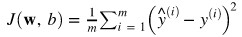
用均方誤差計算訓練集上的損失：

第 3 步(只有在使用梯度下降法訓練時需要):

對每個引數，計算其對損失函式的偏導數：

所有偏導數的梯度計算如下：

第 4 步(只有在使用梯度下降法訓練時需要）:

更新權重向量和偏置量：

其中，表示學習率。

In [4]:

import numpy as np
import matplotlib.pyplot as plt
from sklearn.model_selection import train_test_split
np.random.seed(123)

資料集

In [5]:

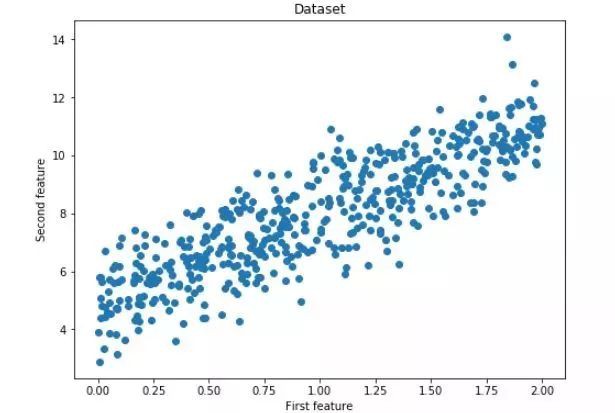
# We will use a simple training set
X = 2 * np.random.rand(500, 1)
y = 5 + 3 * X + np.random.randn(500, 1)
fig = plt.figure(figsize=(8,6))
plt.scatter(X, y)
plt.title("Dataset")
plt.xlabel("First feature")
plt.ylabel("Second feature")
plt.show()

In [6]:

# Split the data into a training and test set
X_train, X_test, y_train, y_test = train_test_split(X, y)
print(f'Shape X_train: {X_train.shape}')
print(f'Shape y_train: {y_train.shape}')
print(f'Shape X_test: {X_test.shape}')
print(f'Shape y_test: {y_test.shape}')

Shape X_train: (375, 1)
Shape y_train: (375, 1)
Shape X_test: (125, 1)
Shape y_test: (125, 1)

線性回歸分類

In [23]:

class LinearRegression:
    
    def __init__(self):
        pass
    
    def train_gradient_descent(self, X, y, learning_rate=0.01, n_iters=100):
        """
        Trains a linear regression model using gradient descent
        """
        # Step 0: Initialize the parameters
        n_samples, n_features = X.shape
        self.weights = np.zeros(shape=(n_features,1))
        self.bias = 0
        costs = []
        
        for i in range(n_iters):
            # Step 1: Compute a linear combination of the input features and weights
            y_predict = np.dot(X, self.weights) + self.bias
           
            # Step 2: Compute cost over training set
            cost = (1 / n_samples) * np.sum((y_predict - y)**2)
            costs.append(cost)
           
            if i % 100 == 0:
                print(f"Cost at iteration {i}: {cost}")
            
            # Step 3: Compute the gradients
            dJ_dw = (2 / n_samples) * np.dot(X.T, (y_predict - y))
            dJ_db = (2 / n_samples) * np.sum((y_predict - y)) 
            
            # Step 4: Update the parameters
            self.weights = self.weights - learning_rate * dJ_dw
            self.bias = self.bias - learning_rate * dJ_db
        
        return self.weights, self.bias, costs
   
    def train_normal_equation(self, X, y):
        """
        Trains a linear regression model using the normal equation
        """
        self.weights = np.dot(np.dot(np.linalg.inv(np.dot(X.T, X)), X.T), y)
        self.bias = 0
        
        return self.weights, self.bias
        
    def predict(self, X):
        return np.dot(X, self.weights) + self.bias

使用梯度下降進行訓練

In [24]:

regressor = LinearRegression()
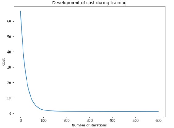
w_trained, b_trained, costs = regressor.train_gradient_descent(X_train, y_train, learning_rate=0.005, n_iters=600)
fig = plt.figure(figsize=(8,6))
plt.plot(np.arange(n_iters), costs)
plt.title("Development of cost during training")
plt.xlabel("Number of iterations")
plt.ylabel("Cost")
plt.show()

Cost at iteration 0: 66.45256981003433 Cost at iteration 100: 2.2084346146095934 Cost at iteration 200: 1.2797812854182806 Cost at iteration 300: 1.2042189195356685 Cost at iteration 400: 1.1564867816573 Cost at iteration 500: 1.121391041394467

測試（梯度下降模型）

In [28]:

n_samples, _ = X_train.shape
n_samples_test, _ = X_test.shape

y_p_train = regressor.predict(X_train)
y_p_test = regressor.predict(X_test)

error_train =  (1 / n_samples) * np.sum((y_p_train - y_train) ** 2)
error_test =  (1 / n_samples_test) * np.sum((y_p_test - y_test) ** 2)

print(f"Error on training set: {np.round(error_train, 4)}")
print(f"Error on test set: {np.round(error_test)}")

Error on training set: 1.0955

Error on test set: 1.0

使用正規方程（normal equation）訓練

# To compute the parameters using the normal equation, we add a bias value of 1 to each input example
X_b_train = np.c_[np.ones((n_samples)), X_train]
X_b_test = np.c_[np.ones((n_samples_test)), X_test]

reg_normal = LinearRegression()
w_trained = reg_normal.train_normal_equation(X_b_train, y_train)

測試（正規方程模型）

y_p_train = reg_normal.predict(X_b_train)
y_p_test = reg_normal.predict(X_b_test)

error_train =  (1 / n_samples) * np.sum((y_p_train - y_train) ** 2)
error_test =  (1 / n_samples_test) * np.sum((y_p_test - y_test) ** 2)

print(f"Error on training set: {np.round(error_train, 4)}")
print(f"Error on test set: {np.round(error_test, 4)}")

Error on training set: 1.0228

Error on test set: 1.0432

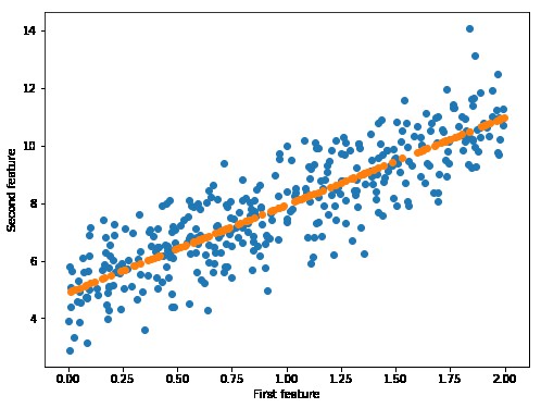
視覺化測試預測

# Plot the test predictions


fig = plt.figure(figsize=(8,6))
plt.scatter(X_train, y_train)
plt.scatter(X_test, y_p_test)
plt.xlabel("First feature")
plt.ylabel("Second feature")
plt.show()

02 Logistic 回歸演演算法

在 Logistic 回歸中，我們試圖對給定輸入特徵的線性組合進行建模，來得到其二元變數的輸出結果。例如，我們可以嘗試使用競選候選人花費的金錢和時間資訊來預測選舉的結果(勝或負)。Logistic 回歸演演算法的工作原理如下。

給定：

資料集
是d-維向量
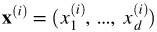
是一個二元的標的變數

Logistic 回歸模型可以理解為一個非常簡單的神經網路：

它有一個實值加權向量
它有一個實值偏置量 b
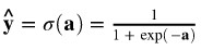
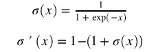
它使用 sigmoid 函式作為其啟用函式

與線性回歸不同，Logistic 回歸沒有封閉解。但由於損失函式是凸函式，因此我們可以使用梯度下降法來訓練模型。事實上，在保證學習速率足夠小且使用足夠的訓練迭代步數的前提下，梯度下降法(或任何其他最佳化演演算法)可以是能夠找到全域性最小值。

訓練 Logistic 回歸模型有不同的步驟。首先(在步驟 0 中)，模型的引數將被初始化。在達到指定訓練次數或引數收斂前，重覆以下其他步驟。

第 0 步：用 0 (或小的隨機值)來初始化權重向量和偏置值

第 1 步：計算輸入的特徵與權重值的線性組合，這可以透過向量化和向量傳播來對所有訓練樣本進行處理：

其中 X 是所有訓練樣本的維度矩陣，其形式為；·表示點積。

第 2 步：用 sigmoid 函式作為啟用函式，其傳回值介於0到1之間：

第 3 步：計算整個訓練集的損失值。

我們希望模型得到的標的值機率落在 0 到 1 之間。因此在訓練期間，我們希望調整引數，使得模型較大的輸出值對應正標簽(真實標簽為 1)，較小的輸出值對應負標簽(真實標簽為 0 )。這在損失函式中表現為如下形式：

第 4 步：對權重向量和偏置量，計算其對損失函式的梯度。

關於這個導數實現的詳細解釋，可以參見這裡（https://stats.stackexchange.com/questions/278771/how-is-the-cost-function-from-logistic-regression-derivated）。

一般形式如下：

對於偏置量的導數計算，此時為 1。

第 5 步：更新權重和偏置值。

其中，表示學習率。

In [24]:

import numpy as np
from sklearn.model_selection import train_test_split
from sklearn.datasets import make_blobs
import matplotlib.pyplot as plt
np.random.seed(123)

% matplotlib inline

資料集

In [25]:

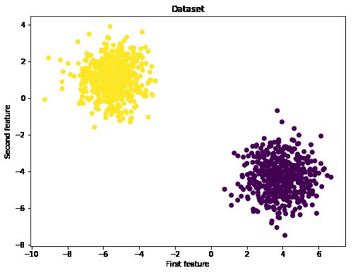
# We will perform logistic regression using a simple toy dataset of two classes
X, y_true = make_blobs(n_samples= 1000, centers=2)

fig = plt.figure(figsize=(8,6))
plt.scatter(X[:,0], X[:,1], c=y_true)
plt.title("Dataset")
plt.xlabel("First feature")
plt.ylabel("Second feature")
plt.show()

In [26]:

# Reshape targets to get column vector with shape (n_samples, 1)
y_true = y_true[:, np.newaxis]
# Split the data into a training and test set
X_train, X_test, y_train, y_test = train_test_split(X, y_true)
print(f'Shape X_train: {X_train.shape}')
print(f'Shape y_train: {y_train.shape}')
print(f'Shape X_test: {X_test.shape}')
print(f'Shape y_test: {y_test.shape}')

Shape X_train: (750, 2)

Shape y_train: (750, 1)

Shape X_test: (250, 2)

Shape y_test: (250, 1)

Logistic回歸分類

In [27]:

class LogisticRegression:
   
    def __init__(self):
        pass

    def sigmoid(self, a):
        return 1 / (1 + np.exp(-a))

    def train(self, X, y_true, n_iters, learning_rate):
        """
        Trains the logistic regression model on given data X and targets y
        """
        # Step 0: Initialize the parameters
        n_samples, n_features = X.shape
        self.weights = np.zeros((n_features, 1))
        self.bias = 0
        costs = []
    
        for i in range(n_iters):
            # Step 1 and 2: Compute a linear combination of the input features and weights, 
            # apply the sigmoid activation function
            y_predict = self.sigmoid(np.dot(X, self.weights) + self.bias)
       
            # Step 3: Compute the cost over the whole training set.
            cost = (- 1 / n_samples) * np.sum(y_true * np.log(y_predict) + (1 - y_true) * (np.log(1 - y_predict)))

            # Step 4: Compute the gradients
            dw = (1 / n_samples) * np.dot(X.T, (y_predict - y_true))
            db = (1 / n_samples) * np.sum(y_predict - y_true)

            # Step 5: Update the parameters
            self.weights = self.weights - learning_rate * dw
            self.bias = self.bias - learning_rate * db

            costs.append(cost)
            if i % 100 == 0:
                print(f"Cost after iteration {i}: {cost}")

        return self.weights, self.bias, costs

    def predict(self, X):
        """
        Predicts binary labels for a set of examples X.
        """
        y_predict = self.sigmoid(np.dot(X, self.weights) + self.bias)
        y_predict_labels = [1 if elem > 0.5 else 0 for elem in y_predict]

        return np.array(y_predict_labels)[:, np.newaxis]

初始化並訓練模型

In [29]:

regressor = LogisticRegression()
w_trained, b_trained, costs = regressor.train(X_train, y_train, n_iters=600, learning_rate=0.009)

fig = plt.figure(figsize=(8,6))
plt.plot(np.arange(600), costs)
plt.title("Development of cost over training")
plt.xlabel("Number of iterations")
plt.ylabel("Cost")
plt.show()

Cost after iteration 0: 0.6931471805599453

Cost after iteration 100: 0.046514002935609956

Cost after iteration 200: 0.02405337743999163

Cost after iteration 300: 0.016354408151412207

Cost after iteration 400: 0.012445770521974634

Cost after iteration 500: 0.010073981792906512

測試模型

In [31]:

y_p_train = regressor.predict(X_train)
y_p_test = regressor.predict(X_test)

print(f"train accuracy: {100 - np.mean(np.abs(y_p_train - y_train)) * 100}%")
print(f"test accuracy: {100 - np.mean(np.abs(y_p_test - y_test))}%")

train accuracy: 100.0%

test accuracy: 100.0%

03 感知器演演算法

感知器是一種簡單的監督式的機器學習演演算法，也是最早的神經網路體系結構之一。它由 Rosenblatt 在 20 世紀 50 年代末提出。感知器是一種二元的線性分類器，其使用 d- 維超平面來將一組訓練樣本( d- 維輸入向量)對映成二進位制輸出值。它的原理如下：

給定：

資料集
是d-維向量
是一個標的變數，它是一個標量

感知器可以理解為一個非常簡單的神經網路：

它有一個實值加權向量
它有一個實值偏置量 b
它使用 Heaviside step 函式作為其啟用函式

感知器的訓練可以使用梯度下降法，訓練演演算法有不同的步驟。首先(在步驟0中)，模型的引數將被初始化。在達到指定訓練次數或引數收斂前，重覆以下其他步驟。

第 0 步：用 0 (或小的隨機值)來初始化權重向量和偏置值

第 1 步：計算輸入的特徵與權重值的線性組合，這可以透過向量化和向量傳播法則來對所有訓練樣本進行處理：

其中 X 是所有訓練示例的維度矩陣，其形式為；·表示點積。

第 2 步：用 Heaviside step 函式作為啟用函式，其傳回一個二進位制值：

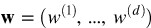
第 3 步：使用感知器的學習規則來計算權重向量和偏置量的更新值。

其中，表示學習率。

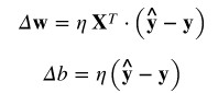
第 4 步：更新權重向量和偏置量。

In [1]:

import numpy as np
import matplotlib.pyplot as plt
from sklearn.datasets import make_blobs
from sklearn.model_selection import train_test_split
np.random.seed(123)

% matplotlib inline

資料集

In [2]:

X, y = make_blobs(n_samples=1000, centers=2)
fig = plt.figure(figsize=(8,6))
plt.scatter(X[:,0], X[:,1], c=y)
plt.title("Dataset")
plt.xlabel("First feature")
plt.ylabel("Second feature")
plt.show()

In [3]:

y_true = y[:, np.newaxis]

X_train, X_test, y_train, y_test = train_test_split(X, y_true)
print(f'Shape X_train: {X_train.shape}')
print(f'Shape y_train: {y_train.shape})')
print(f'Shape X_test: {X_test.shape}')
print(f'Shape y_test: {y_test.shape}')

Shape X_train: (750, 2)

Shape y_train: (750, 1))

Shape X_test: (250, 2)

Shape y_test: (250, 1)

感知器分類

In [6]:

class Perceptron():

    def __init__(self):
        pass

    def train(self, X, y, learning_rate=0.05, n_iters=100):
        n_samples, n_features = X.shape

        # Step 0: Initialize the parameters
        self.weights = np.zeros((n_features,1))
        self.bias = 0

        for i in range(n_iters):
            # Step 1: Compute the activation
            a = np.dot(X, self.weights) + self.bias

            # Step 2: Compute the output
            y_predict = self.step_function(a)

            # Step 3: Compute weight updates
            delta_w = learning_rate * np.dot(X.T, (y - y_predict))
            delta_b = learning_rate * np.sum(y - y_predict)

            # Step 4: Update the parameters
            self.weights += delta_w
            self.bias += delta_b

        return self.weights, self.bias

    def step_function(self, x):
        return np.array([1 if elem >= 0 else 0 for elem in x])[:, np.newaxis]

    def predict(self, X):
        a = np.dot(X, self.weights) + self.bias
        return self.step_function(a)

初始化並訓練模型

In [7]:

p = Perceptron()
w_trained, b_trained = p.train(X_train, y_train,learning_rate=0.05, n_iters=500)

測試

In [10]:

y_p_train = p.predict(X_train)
y_p_test = p.predict(X_test)

print(f"training accuracy: {100 - np.mean(np.abs(y_p_train - y_train)) * 100}%")
print(f"test accuracy: {100 - np.mean(np.abs(y_p_test - y_test)) * 100}%")

training accuracy: 100.0%

test accuracy: 100.0%

視覺化決策邊界

In [13]:

def plot_hyperplane(X, y, weights, bias):
    """
    Plots the dataset and the estimated decision hyperplane
    """
    slope = - weights[0]/weights[1]
    intercept = - bias/weights[1]
    x_hyperplane = np.linspace(-10,10,10)
    y_hyperplane = slope * x_hyperplane + intercept
    fig = plt.figure(figsize=(8,6))
    plt.scatter(X[:,0], X[:,1], c=y)
    plt.plot(x_hyperplane, y_hyperplane, '-')
    plt.title("Dataset and fitted decision hyperplane")
    plt.xlabel("First feature")
    plt.ylabel("Second feature")
    plt.show()

In [14]:

plot_hyperplane(X, y, w_trained, b_trained)

04 K 最近鄰演演算法

k-nn 演演算法是一種簡單的監督式的機器學習演演算法，可以用於解決分類和回歸問題。這是一個基於實體的演演算法，並不是估算模型，而是將所有訓練樣本儲存在記憶體中，並使用相似性度量進行預測。

給定一個輸入示例，k-nn 演演算法將從記憶體中檢索 k 個最相似的實體。相似性是根據距離來定義的，也就是說，與輸入示例之間距離最小(歐幾裡得距離)的訓練樣本被認為是最相似的樣本。

輸入示例的標的值計算如下：

分類問題：

a) 不加權：輸出 k 個最近鄰中最常見的分類

b) 加權：將每個分類值的k個最近鄰的權重相加，輸出權重最高的分類

回歸問題：

a) 不加權：輸出k個最近鄰值的平均值

b) 加權：對於所有分類值，將分類值加權求和並將結果除以所有權重的總和

加權版本的 k-nn 演演算法是改進版本，其中每個近鄰的貢獻值根據其與查詢點之間的距離進行加權。下麵，我們在 sklearn 用 k-nn 演演算法的原始版本實現數字資料集的分類。

In [1]:

import numpy as np
import matplotlib.pyplot as plt
from sklearn.datasets import load_digits
from sklearn.model_selection import train_test_split
np.random.seed(123)

% matplotlib inline

資料集

In [2]:

# We will use the digits dataset as an example. It consists of the 1797 images of hand-written digits. Each digit is
# represented by a 64-dimensional vector of pixel values.


digits = load_digits()
X, y = digits.data, digits.target

X_train, X_test, y_train, y_test = train_test_split(X, y)
print(f'X_train shape: {X_train.shape}')
print(f'y_train shape: {y_train.shape}')
print(f'X_test shape: {X_test.shape}')
print(f'y_test shape: {y_test.shape}')

# Example digits
fig = plt.figure(figsize=(10,8))
for i in range(10):
    ax = fig.add_subplot(2, 5, i+1)
    plt.imshow(X[i].reshape((8,8)), cmap='gray')

X_train shape: (1347, 64)

y_train shape: (1347,)

X_test shape: (450, 64)

y_test shape: (450,)

K 最鄰近類別

In [3]:

class kNN():
    def __init__(self):
        pass

    def fit(self, X, y):
        self.data = X
        self.targets = y

    def euclidean_distance(self, X):
        """
        Computes the euclidean distance between the training data and
        a new input example or matrix of input examples X
        """
        # input: single data point
        if X.ndim == 1:
            l2 = np.sqrt(np.sum((self.data - X)**2, axis=1))

        # input: matrix of data points
        if X.ndim == 2:
            n_samples, _ = X.shape
            l2 = [np.sqrt(np.sum((self.data - X[i])**2, axis=1)) for i in range(n_samples)]

        return np.array(l2)

    def predict(self, X, k=1):
        """
        Predicts the classification for an input example or matrix of input examples X
        """
        # step 1: compute distance between input and training data
        dists = self.euclidean_distance(X)

        # step 2: find the k nearest neighbors and their classifications
        if X.ndim == 1:
            if k == 1:
                nn = np.argmin(dists)
                return self.targets[nn]
            else:
                knn = np.argsort(dists)[:k]
                y_knn = self.targets[knn]
                max_vote = max(y_knn, key=list(y_knn).count)
                return max_vote

        if X.ndim == 2:
            knn = np.argsort(dists)[:, :k]
            y_knn = self.targets[knn]
            if k == 1:
                return y_knn.T
            else:
                n_samples, _ = X.shape
                max_votes = [max(y_knn[i], key=list(y_knn[i]).count) for i in range(n_samples)]
                return max_votes

初始化並訓練模型

In [11]:

knn = kNN()
knn.fit(X_train, y_train)

print("Testing one datapoint, k=1")
print(f"Predicted label: {knn.predict(X_test[0], k=1)}")
print(f"True label: {y_test[0]}")
print()
print("Testing one datapoint, k=5")
print(f"Predicted label: {knn.predict(X_test[20], k=5)}")
print(f"True label: {y_test[20]}")
print()
print("Testing 10 datapoint, k=1")
print(f"Predicted labels: {knn.predict(X_test[5:15], k=1)}")
print(f"True labels: {y_test[5:15]}")
print()
print("Testing 10 datapoint, k=4")
print(f"Predicted labels: {knn.predict(X_test[5:15], k=4)}")
print(f"True labels: {y_test[5:15]}")
print()

Testing one datapoint, k=1

Predicted label: 3

True label: 3

Testing one datapoint, k=5

Predicted label: 9

True label: 9

Testing 10 datapoint, k=1

Predicted labels: [[3 1 0 7 4 0 0 5 1 6]]

True labels: [3 1 0 7 4 0 0 5 1 6]

Testing 10 datapoint, k=4

Predicted labels: [3, 1, 0, 7, 4, 0, 0, 5, 1, 6]

True labels: [3 1 0 7 4 0 0 5 1 6]

測試集精度

In [12]:

# Compute accuracy on test set
y_p_test1 = knn.predict(X_test, k=1)
test_acc1= np.sum(y_p_test1[0] == y_test)/len(y_p_test1[0]) * 100
print(f"Test accuracy with k = 1: {format(test_acc1)}")

y_p_test8 = knn.predict(X_test, k=5)
test_acc8= np.sum(y_p_test8 == y_test)/len(y_p_test8) * 100
print(f"Test accuracy with k = 8: {format(test_acc8)}")

Test accuracy with k = 1: 97.77777777777777

Test accuracy with k = 8: 97.55555555555556

05 K均值聚類演演算法

K-Means 是一種非常簡單的聚類演演算法(聚類演演算法都屬於無監督學習)。給定固定數量的聚類和輸入資料集，該演演算法試圖將資料劃分為聚類，使得聚類內部具有較高的相似性，聚類與聚類之間具有較低的相似性。

演演算法原理

1. 初始化聚類中心，或者在輸入資料範圍內隨機選擇，或者使用一些現有的訓練樣本(推薦)

2. 直到收斂

將每個資料點分配到最近的聚類。點與聚類中心之間的距離是透過歐幾裡德距離測量得到的。
透過將聚類中心的當前估計值設定為屬於該聚類的所有實體的平均值，來更新它們的當前估計值。

標的函式

聚類演演算法的標的函式試圖找到聚類中心，以便資料將劃分到相應的聚類中，並使得資料與其最接近的聚類中心之間的距離盡可能小。

給定一組資料X1，…，Xn和一個正數k，找到k個聚類中心C1，…，Ck並最小化標的函式：

這裡：

決定了資料點是否屬於類
表示類的聚類中心
表示歐幾裡得距離

K-Means 演演算法的缺點：

聚類的個數在開始就要設定
聚類的結果取決於初始設定的聚類中心
對異常值很敏感
不適合用於發現非凸聚類問題
該演演算法不能保證能夠找到全域性最優解，因此它往往會陷入一個區域性最優解

In [21]:

import numpy as np
import matplotlib.pyplot as plt
import random
from sklearn.datasets import make_blobs
np.random.seed(123)

% matplotlib inline

資料集

In [22]:

X, y = make_blobs(centers=4, n_samples=1000)
print(f'Shape of dataset: {X.shape}')

fig = plt.figure(figsize=(8,6))
plt.scatter(X[:,0], X[:,1], c=y)
plt.title("Dataset with 4 clusters")
plt.xlabel("First feature")
plt.ylabel("Second feature")
plt.show()

Shape of dataset: (1000, 2)

K均值分類

In [23]:

class KMeans():
    def __init__(self, n_clusters=4):
        self.k = n_clusters

    def fit(self, data):
        """
        Fits the k-means model to the given dataset
        """
        n_samples, _ = data.shape
        # initialize cluster centers
        self.centers = np.array(random.sample(list(data), self.k))
        self.initial_centers = np.copy(self.centers)

        # We will keep track of whether the assignment of data points
        # to the clusters has changed. If it stops changing, we are 
        # done fitting the model
        old_assigns = None
        n_iters = 0

        while True:
            new_assigns = [self.classify(datapoint) for datapoint in data]

            if new_assigns == old_assigns:
                print(f"Training finished after {n_iters} iterations!")
                return

            old_assigns = new_assigns
            n_iters += 1

            # recalculate centers
            for id_ in range(self.k):
                points_idx = np.where(np.array(new_assigns) == id_)
                datapoints = data[points_idx]
                self.centers[id_] = datapoints.mean(axis=0)

    def l2_distance(self, datapoint):
        dists = np.sqrt(np.sum((self.centers - datapoint)**2, axis=1))
        return dists

    def classify(self, datapoint):
        """
        Given a datapoint, compute the cluster closest to the
        datapoint. Return the cluster ID of that cluster.
        """
        dists = self.l2_distance(datapoint)
        return np.argmin(dists)

    def plot_clusters(self, data):
        plt.figure(figsize=(12,10))
        plt.title("Initial centers in black, final centers in red")
        plt.scatter(data[:, 0], data[:, 1], marker='.', c=y)
        plt.scatter(self.centers[:, 0], self.centers[:,1], c='r')
        plt.scatter(self.initial_centers[:, 0], self.initial_centers[:,1], c='k')
        plt.show()

初始化並調整模型

kmeans = KMeans(n_clusters=4)
kmeans.fit(X)

Training finished after 4 iterations!

描繪初始和最終的聚類中心

kmeans.plot_clusters(X)

06 簡單的神經網路

在這一章節裡，我們將實現一個簡單的神經網路架構，將 2 維的輸入向量對映成二進位制輸出值。我們的神經網路有 2 個輸入神經元，含 6 個隱藏神經元隱藏層及 1 個輸出神經元。

我們將透過層之間的權重矩陣來表示神經網路結構。在下麵的例子中，輸入層和隱藏層之間的權重矩陣將被表示為，隱藏層和輸出層之間的權重矩陣為。除了連線神經元的權重向量外，每個隱藏和輸出的神經元都會有一個大小為 1 的偏置量。

我們的訓練集由 m = 750 個樣本組成。因此，我們的矩陣維度如下：

訓練集維度： X = (750，2)
標的維度： Y = (750，1)
維度：(m，nhidden) = (2,6)
維度：(bias vector)：(1，nhidden) = (1,6)
維度： (nhidden，noutput)= (6,1)
維度：(bias vector)：(1，noutput) = (1,1)

損失函式

我們使用與 Logistic 回歸演演算法相同的損失函式：

對於多類別的分類任務，我們將使用這個函式的通用形式作為損失函式，稱之為分類交叉熵函式。

訓練

我們將用梯度下降法來訓練我們的神經網路，並透過反向傳播法來計算所需的偏導數。訓練過程主要有以下幾個步驟：

1. 初始化引數(即權重量和偏差量)

2. 重覆以下過程，直到收斂：

透過網路傳播當前輸入的批次大小，並計算所有隱藏和輸出單元的啟用值和輸出值。
針對每個引數計算其對損失函式的偏導數
更新引數

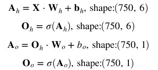
前向傳播過程

首先，我們計算網路中每個單元的啟用值和輸出值。為了加速這個過程的實現，我們不會單獨為每個輸入樣本執行此操作，而是透過向量化對所有樣本一次性進行處理。其中：

表示對所有訓練樣本啟用隱層單元的矩陣
表示對所有訓練樣本輸出隱層單位的矩陣

隱層神經元將使用 tanh 函式作為其啟用函式：

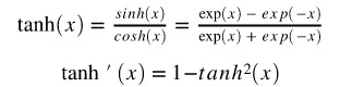
輸出層神經元將使用 sigmoid 函式作為啟用函式：

啟用值和輸出值計算如下(·表示點乘)：

反向傳播過程

為了計算權重向量的更新值，我們需要計算每個神經元對損失函式的偏導數。這裡不會給出這些公式的推導，你會在其他網站上找到很多更好的解釋(https://mattmazur.com/2015/03/17/a-step-by-step-backpropagation-example/)。

對於輸出神經元，梯度計算如下(矩陣符號)：

對於輸入和隱層的權重矩陣，梯度計算如下：

權重更新

In [3]:

import numpy as np
import pandas as pd
import matplotlib.pyplot as plt
from sklearn.datasets import make_circles
from sklearn.model_selection import train_test_split
np.random.seed(123)
% matplotlib inline

資料集

In [4]:

X, y = make_circles(n_samples=1000, factor=0.5, noise=.1)
fig = plt.figure(figsize=(8,6))
plt.scatter(X[:,0], X[:,1], c=y)
plt.xlim([-1.5, 1.5])
plt.ylim([-1.5, 1.5])
plt.title("Dataset")
plt.xlabel("First feature")
plt.ylabel("Second feature")
plt.show()

In [5]:

# reshape targets to get column vector with shape (n_samples, 1)
y_true = y[:, np.newaxis]
# Split the data into a training and test set
X_train, X_test, y_train, y_test = train_test_split(X, y_true)
print(f'Shape X_train: {X_train.shape}')
print(f'Shape y_train: {y_train.shape}')
print(f'Shape X_test: {X_test.shape}')
print(f'Shape y_test: {y_test.shape}')

Shape X_train: (750, 2)

Shape y_train: (750, 1)

Shape X_test: (250, 2)

Shape y_test: (250, 1)

Neural Network Class

以下部分實現受益於吳恩達的課程

https://www.coursera.org/learn/neural-networks-deep-learning

class NeuralNet():
    def __init__(self, n_inputs, n_outputs, n_hidden):
        self.n_inputs = n_inputs
        self.n_outputs = n_outputs
        self.hidden = n_hidden
        # Initialize weight matrices and bias vectors
        self.W_h = np.random.randn(self.n_inputs, self.hidden)
        self.b_h = np.zeros((1, self.hidden))
        self.W_o = np.random.randn(self.hidden, self.n_outputs)
        self.b_o = np.zeros((1, self.n_outputs))
    def sigmoid(self, a):
        return 1 / (1 + np.exp(-a))
    def forward_pass(self, X):
        """
        Propagates the given input X forward through the net.
        Returns:
            A_h: matrix with activations of all hidden neurons for all input examples
            O_h: matrix with outputs of all hidden neurons for all input examples
            A_o: matrix with activations of all output neurons for all input examples
            O_o: matrix with outputs of all output neurons for all input examples
        """
        # Compute activations and outputs of hidden units
        A_h = np.dot(X, self.W_h) + self.b_h
        O_h = np.tanh(A_h)
        # Compute activations and outputs of output units
        A_o = np.dot(O_h, self.W_o) + self.b_o
        O_o = self.sigmoid(A_o)
        outputs = {
                "A_h": A_h,
                "A_o": A_o,
                "O_h": O_h,
                "O_o": O_o,
                }
        return outputs
    def cost(self, y_true, y_predict, n_samples):
        """
        Computes and returns the cost over all examples
        """
        # same cost function as in logistic regression
        cost = (- 1 / n_samples) * np.sum(y_true * np.log(y_predict) + (1 - y_true) * (np.log(1 - y_predict)))
        cost = np.squeeze(cost)
        assert isinstance(cost, float)
        return cost
    def backward_pass(self,  X, Y, n_samples, outputs):
        """
        Propagates the errors backward through the net.
        Returns:
            dW_h: partial derivatives of loss function w.r.t hidden weights
            db_h: partial derivatives of loss function w.r.t hidden bias
            dW_o: partial derivatives of loss function w.r.t output weights
            db_o: partial derivatives of loss function w.r.t output bias
        """
        dA_o = (outputs["O_o"] - Y)
        dW_o = (1 / n_samples) * np.dot(outputs["O_h"].T, dA_o)
        db_o = (1 / n_samples) * np.sum(dA_o)
        dA_h = (np.dot(dA_o, self.W_o.T)) * (1 - np.power(outputs["O_h"], 2))
        dW_h = (1 / n_samples) * np.dot(X.T, dA_h)
        db_h = (1 / n_samples) * np.sum(dA_h)
        gradients = {
                "dW_o": dW_o,
                "db_o": db_o,
                "dW_h": dW_h,
                "db_h": db_h,
                }
        return gradients
    def update_weights(self, gradients, eta):
        """
        Updates the model parameters using a fixed learning rate
        """
        self.W_o = self.W_o - eta * gradients["dW_o"]
        self.W_h = self.W_h - eta * gradients["dW_h"]
        self.b_o = self.b_o - eta * gradients["db_o"]
        self.b_h = self.b_h - eta * gradients["db_h"]
    def train(self, X, y, n_iters=500, eta=0.3):
        """
        Trains the neural net on the given input data
        """
        n_samples, _ = X.shape
        for i in range(n_iters):
            outputs = self.forward_pass(X)
            cost = self.cost(y, outputs["O_o"], n_samples=n_samples)
            gradients = self.backward_pass(X, y, n_samples, outputs)
            if i % 100 == 0:
                print(f'Cost at iteration {i}: {np.round(cost, 4)}')
            self.update_weights(gradients, eta)
    def predict(self, X):
        """
        Computes and returns network predictions for given dataset
        """
        outputs = self.forward_pass(X)
        y_pred = [1 if elem >= 0.5 else 0 for elem in outputs["O_o"]]
        return np.array(y_pred)[:, np.newaxis]

初始化並訓練神經網路

nn = NeuralNet(n_inputs=2, n_hidden=6, n_outputs=1)
print("Shape of weight matrices and bias vectors:")
print(f'W_h shape: {nn.W_h.shape}')
print(f'b_h shape: {nn.b_h.shape}')
print(f'W_o shape: {nn.W_o.shape}')
print(f'b_o shape: {nn.b_o.shape}')
print()
print("Training:")
nn.train(X_train, y_train, n_iters=2000, eta=0.7)

Shape of weight matrices and bias vectors:

W_h shape: (2, 6)

b_h shape: (1, 6)

W_o shape: (6, 1)

b_o shape: (1, 1)

Training:

Cost at iteration 0: 1.0872

Cost at iteration 100: 0.2723

Cost at iteration 200: 0.1712

Cost at iteration 300: 0.1386

Cost at iteration 400: 0.1208

Cost at iteration 500: 0.1084

Cost at iteration 600: 0.0986

Cost at iteration 700: 0.0907

Cost at iteration 800: 0.0841

Cost at iteration 900: 0.0785

Cost at iteration 1000: 0.0739

Cost at iteration 1100: 0.0699

Cost at iteration 1200: 0.0665

Cost at iteration 1300: 0.0635

Cost at iteration 1400: 0.061

Cost at iteration 1500: 0.0587

Cost at iteration 1600: 0.0566

Cost at iteration 1700: 0.0547

Cost at iteration 1800: 0.0531

Cost at iteration 1900: 0.0515

測試神經網路

n_test_samples, _ = X_test.shape
y_predict = nn.predict(X_test)
print(f"Classification accuracy on test set: {(np.sum(y_predict == y_test)/n_test_samples)*100} %")

Classification accuracy on test set: 98.4 %

視覺化決策邊界

X_temp, y_temp = make_circles(n_samples=60000, noise=.5)
y_predict_temp = nn.predict(X_temp)
y_predict_temp = np.ravel(y_predict_temp)

fig = plt.figure(figsize=(8,12))
ax = fig.add_subplot(2,1,1)
plt.scatter(X[:,0], X[:,1], c=y)
plt.xlim([-1.5, 1.5])
plt.ylim([-1.5, 1.5])
plt.xlabel("First feature")
plt.ylabel("Second feature")
plt.title("Training and test set")
ax = fig.add_subplot(2,1,2)
plt.scatter(X_temp[:,0], X_temp[:,1], c=y_predict_temp)
plt.xlim([-1.5, 1.5])
plt.ylim([-1.5, 1.5])
plt.xlabel("First feature")
plt.ylabel("Second feature")
plt.title("Decision boundary")

Out[11]:Text(0.5,1,’Decision boundary’)

07 Softmax 回歸演演算法

Softmax 回歸演演算法，又稱為多項式或多類別的 Logistic 回歸演演算法。

給定：

資料集

是d-維向量
是對應於的標的變數，例如對於K=3分類問題，

Softmax 回歸模型有以下幾個特點：

對於每個類別，都存在一個獨立的、實值加權向量
這個權重向量通常作為權重矩陣中的行。
對於每個類別，都存在一個獨立的、實值偏置量b
它使用 softmax 函式作為其啟用函式
它使用交叉熵( cross-entropy )作為損失函式

訓練 Softmax 回歸模型有不同步驟。首先(在步驟0中)，模型的引數將被初始化。在達到指定訓練次數或引數收斂前，重覆以下其他步驟。

第 0 步：用 0 (或小的隨機值)來初始化權重向量和偏置值

第 1 步：對於每個類別k，計算其輸入的特徵與權重值的線性組合，也就是說為每個類別的訓練樣本計算一個得分值。對於類別k，輸入向量為,則得分值的計算如下：

其中表示類別k的權重矩陣，·表示點積。

我們可以透過向量化和向量傳播法則計算所有類別及其訓練樣本的得分值：

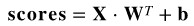
其中 X 是所有訓練樣本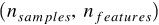的維度矩陣，W 表示每個類別的權重矩陣維度，其形式為；

第 2 步：用 softmax 函式作為啟用函式，將得分值轉化為機率值形式。屬於類別 k 的輸入向量的機率值為：

同樣地，我們可以透過向量化來對所有類別同時處理，得到其機率輸出。模型預測出的表示的是該類別的最高機率。

第 3 步：計算整個訓練集的損失值。

我們希望模型預測出的高機率值是標的類別，而低機率值表示其他類別。這可以透過以下的交叉熵損失函式來實現：

在上面公式中，標的類別標簽表示成獨熱編碼形式( one-hot )。因此為1時表示的標的類別是 k，反之則為 0。

第 4 步：對權重向量和偏置量，計算其對損失函式的梯度。

關於這個導數實現的詳細解釋，可以參見這裡（http://ufldl.stanford.edu/tutorial/supervised/SoftmaxRegression/）。

一般形式如下：

對於偏置量的導數計算，此時為1。

第 5 步：對每個類別k，更新其權重和偏置值。

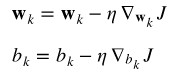
其中，表示學習率。

In [1]:

from sklearn.datasets import load_iris
import numpy as np
from sklearn.model_selection import train_test_split
from sklearn.datasets import make_blobs
import matplotlib.pyplot as plt
np.random.seed(13)

資料集

In [2]:

X, y_true = make_blobs(centers=4, n_samples = 5000)
fig = plt.figure(figsize=(8,6))
plt.scatter(X[:,0], X[:,1], c=y_true)
plt.title("Dataset")
plt.xlabel("First feature")
plt.ylabel("Second feature")
plt.show()

In [3]:

# reshape targets to get column vector with shape (n_samples, 1)
y_true = y_true[:, np.newaxis]
# Split the data into a training and test set
X_train, X_test, y_train, y_test = train_test_split(X, y_true)
print(f'Shape X_train: {X_train.shape}')
print(f'Shape y_train: {y_train.shape}')
print(f'Shape X_test: {X_test.shape}')
print(f'Shape y_test: {y_test.shape}')

Shape X_train: (3750, 2)

Shape y_train: (3750, 1)

Shape X_test: (1250, 2)

Shape y_test: (1250, 1)

Softmax回歸分類

class SoftmaxRegressor:
    def __init__(self):
        pass
    def train(self, X, y_true, n_classes, n_iters=10, learning_rate=0.1):
        """
        Trains a multinomial logistic regression model on given set of training data
        """
        self.n_samples, n_features = X.shape
        self.n_classes = n_classes
        self.weights = np.random.rand(self.n_classes, n_features)
        self.bias = np.zeros((1, self.n_classes))
        all_losses = []
        for i in range(n_iters):
            scores = self.compute_scores(X)
            probs = self.softmax(scores)
            y_predict = np.argmax(probs, axis=1)[:, np.newaxis]
            y_one_hot = self.one_hot(y_true)
            loss = self.cross_entropy(y_one_hot, probs)
            all_losses.append(loss)
            dw = (1 / self.n_samples) * np.dot(X.T, (probs - y_one_hot))
            db = (1 / self.n_samples) * np.sum(probs - y_one_hot, axis=0)
            self.weights = self.weights - learning_rate * dw.T
            self.bias = self.bias - learning_rate * db
            if i % 100 == 0:
                print(f'Iteration number: {i}, loss: {np.round(loss, 4)}')
        return self.weights, self.bias, all_losses
    def predict(self, X):
        """
        Predict class labels for samples in X.
        Args:
            X: numpy array of shape (n_samples, n_features)
        Returns:
            numpy array of shape (n_samples, 1) with predicted classes
        """
        scores = self.compute_scores(X)
        probs = self.softmax(scores)
        return np.argmax(probs, axis=1)[:, np.newaxis]
    def softmax(self, scores):
        """
        Tranforms matrix of predicted scores to matrix of probabilities
        Args:
            scores: numpy array of shape (n_samples, n_classes)
            with unnormalized scores
        Returns:
            softmax: numpy array of shape (n_samples, n_classes)
            with probabilities
        """
        exp = np.exp(scores)
        sum_exp = np.sum(np.exp(scores), axis=1, keepdims=True)
        softmax = exp / sum_exp
        return softmax
    def compute_scores(self, X):
        """
        Computes class-scores for samples in X
        Args:
            X: numpy array of shape (n_samples, n_features)
        Returns:
            scores: numpy array of shape (n_samples, n_classes)
        """
        return np.dot(X, self.weights.T) + self.bias
    def cross_entropy(self, y_true, scores):
        loss = - (1 / self.n_samples) * np.sum(y_true * np.log(scores))
        return loss
    def one_hot(self, y):
        """
        Tranforms vector y of labels to one-hot encoded matrix
        """
        one_hot = np.zeros((self.n_samples, self.n_classes))
        one_hot[np.arange(self.n_samples), y.T] = 1
        return one_hot

初始化並訓練模型

regressor = SoftmaxRegressor()
w_trained, b_trained, loss = regressor.train(X_train, y_train, learning_rate=0.1, n_iters=800, n_classes=4)
fig = plt.figure(figsize=(8,6))
plt.plot(np.arange(800), loss)
plt.title("Development of loss during training")
plt.xlabel("Number of iterations")
plt.ylabel("Loss")
plt.show()Iteration number: 0, loss: 1.393

Iteration number: 100, loss: 0.2051

Iteration number: 200, loss: 0.1605

Iteration number: 300, loss: 0.1371

Iteration number: 400, loss: 0.121

Iteration number: 500, loss: 0.1087

Iteration number: 600, loss: 0.0989

Iteration number: 700, loss: 0.0909

測試模型

n_test_samples, _ = X_test.shape
y_predict = regressor.predict(X_test)
print(f"Classification accuracy on test set: {(np.sum(y_predict == y_test)/n_test_samples) * 100}%")

測試集分類準確率：99.03999999999999%

編譯：林椿眄

來源：人工智慧頭條（ID：AI_Thinker）