作者根據每週釋出總結的系列文章,彙總了2018年針對資料科學家/AI的最佳庫、repos、包和工具。本文對其進行了梳理,列舉了人工智慧和資料科學的七大Python庫。
本文作者Favio Vázquez從2018年開始釋出《資料科學和人工智慧每週文摘:Python & R》系列文章,為資料科學家介紹最好的庫、repos、packages以及工具。
一年結束,作者列出了2018年的7大最好的Python庫,這些庫確實地改進了研究人員的工作方式。
作者:Favio Vázquez
原文連結:
https://heartbeat.fritz.ai/top-7-libraries-and-packages-of-the-year-for-data-science-and-ai-python-r-6b7cca2bf000

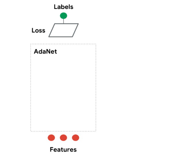
Top7 AdaNet:快速靈活的AutoML框架


(https://github.com/tensorflow/adanet)
AdaNet是一個輕量級的、可擴充套件的TensorFlow AutoML框架,用於使用AdaNet演演算法訓練和部署自適應神經網路[Cortes et al. ICML 2017]。AdaNet結合了多個學習子網路,以減輕設計有效的神經網路所固有的複雜性。
這個軟體包將幫助你選擇最優的神經網路架構,實現一種自適應演演算法,用於學習作為子網路集合的神經架構。
你需要瞭解TensorFlow才能使用這個包,因為它實現了TensorFlow Estimator,但這將透過封裝訓練、評估、預測和匯出服務來幫助你簡化機器學習程式設計。
你可以構建一個神經網路的集合,這個庫將幫助你最佳化一個標的,以平衡集合在訓練集上的效能和將其泛化到未見過資料的能力之間的權衡。
安裝
安裝adanet之前需將TensorFlow升級到1.7或以上:
$ pip install "tensorflow>=1.7.0"
從原始碼安裝
要從原始碼進行安裝,首先需要安裝bazel。
下一步,複製adanet和cd到它的根目錄:
$ git clone https://github.com/tensorflow/adanet && cd adanet
從adanet根目錄執行測試:
$ cd adanet
$ bazel test -c opt //...
確認一切正常後,將adanet安裝為pip包。
現在,可以對adanet進行試驗了。
import adanet
用法
Top6 TPOT:一個自動化的Python機器學習工具

(https://github.com/EpistasisLab/tpot)
TPOT全稱是基於樹的pipeline最佳化工具(Tree-based Pipeline Optimization Tool),這是一個非常棒Python自動機器學習工具,使用遺傳程式設計最佳化機器學習pipeline。
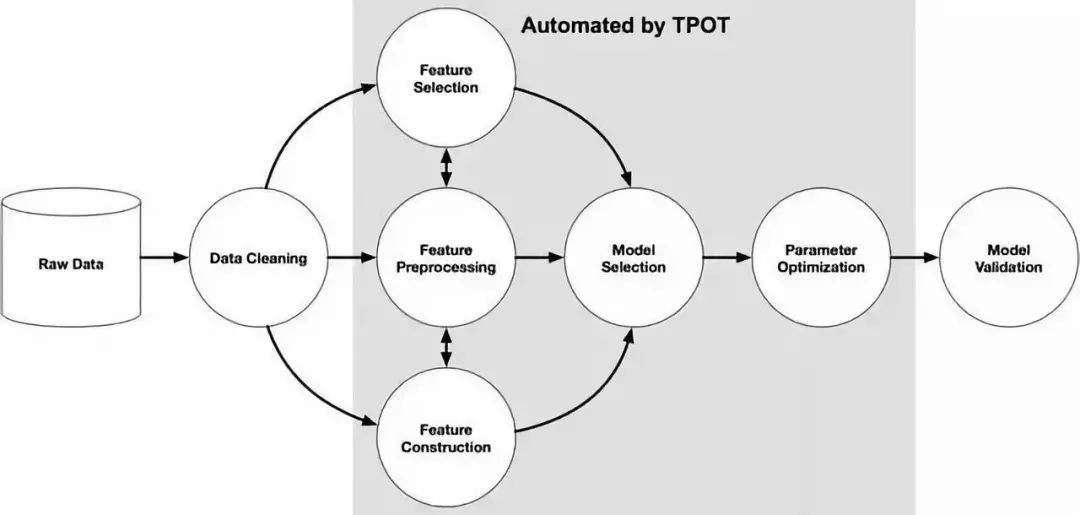
TPOT可以自動化許多東西,包括生命特性選擇、模型選擇、特性構建等等。如果你是Python機器學習者,很幸運,TPOT是構建在Scikit-learn之上的,所以它生成的所有程式碼看起來應該很熟悉。
它的作用是透過智慧地探索數千種可能的pipeline來自動化機器學習中最繁瑣的部分,找到最適合你的資料的pipeline,然後為你提供最佳的 Python 程式碼。
它的工作原理如下:
安裝
執行以下程式碼:
pip install tpot
例子:
首先讓我們從基本的Iris資料集開始:
from tpot import TPOTClassifier
from sklearn.datasets import load_iris
from sklearn.model_selection import train_test_split

# Load iris dataset
iris = load_iris()

# Split the data

X_trainX_train, X_test, y_train, y_test = train_test_split(iris.data, iris.target,
 train_size=0.75, test_size=0.25)

# Fit the TPOT classifier

tpot = TPOTClassifier(verbosity=2, max_time_mins=2)
tpot.fit(X_train, y_train)

# Export the pipeline
tpot.export('tpot_iris_pipeline.py')
(左右滑動可檢視完整程式碼)
我們在這裡構建了一個非常基本的TPOT pipeline,它將嘗試尋找最佳ML pipeline來預測iris.target。然後儲存這個pipeline。之後,我們要做的就非常簡單了——載入生成的.py檔案,你將看到:
import numpy as np
from sklearn.kernel_approximation import RBFSampler
from sklearn.model_selection import train_test_split
from sklearn.pipeline import make_pipeline
from sklearn.tree import DecisionTreeClassifier
# NOTE: Make sure that the class is labeled 'class' in the data file
tpot_data = np.recfromcsv('PATH/TO/DATA/FILE', delimiter='COLUMN_SEPARATOR', dtype=np.float64)
features = np.delete(tpot_data.view(np.float64).reshape(tpot_data.size, -1), tpot_data.dtype.names.index('class'), axis=1)
training_features, testing_features, training_classes, testing_classes =
 train_test_split(features, tpot_data['class'], random_state=42)
exported_pipeline = make_pipeline(
 RBFSampler(gamma=0.8500000000000001),
 DecisionTreeClassifier(criterion="entropy", max_depth=3, min_samples_leaf=4, min_samples_split=9)
)
exported_pipeline.fit(training_features, training_classes)
results = exported_pipeline.predict(testing_features)
(左右滑動可檢視完整程式碼)
就是這樣。你已經以一種簡單但強大的方式為Iris資料集構建一個分類器。
現在我們來看看MNIST的資料集:
from tpot import TPOTClassifier
from sklearn.datasets import load_digits
from sklearn.model_selection import train_test_split

# load and split dataset
digitsdigits == load_digitsload_di ()
X_train, X_test, y_train, y_test = train_test_split(digits.data, digits.target,
 train_size=0.75, test_size=0.25)

# Fit the TPOT classifier
tpot = TPOTClassifier(verbosity=2, max_time_mins=5, population_size=40)
tpot.fit(X_train, y_train)

# Export pipeline
tpot.export('tpot_mnist_pipeline.py')
(左右滑動可檢視完整程式碼)
接下來我們再次載入生成的 .py檔案,你將看到:
import numpy as np
from sklearn.model_selection import train_test_split
from sklearn.neighbors import KNeighborsClassifier
# NOTE: Make sure that the class is labeled 'class' in the data file
tpot_data = np.recfromcsv('PATH/TO/DATA/FILE', delimiter='COLUMN_SEPARATOR', dtype=np.float64)
features = np.delete(tpot_data.view(np.float64).reshape(tpot_data.size, -1), tpot_data.dtype.names.index('class'), axis=1)
training_features, testing_features, training_classes, testing_classes =
 train_test_split(features, tpot_data['class'], random_state=42)
exported_pipeline = KNeighborsClassifier(n_neighbors=4, p=2, weights="distance")
exported_pipeline.fit(training_features, training_classes)
results = exported_pipeline.predict(testing_features)
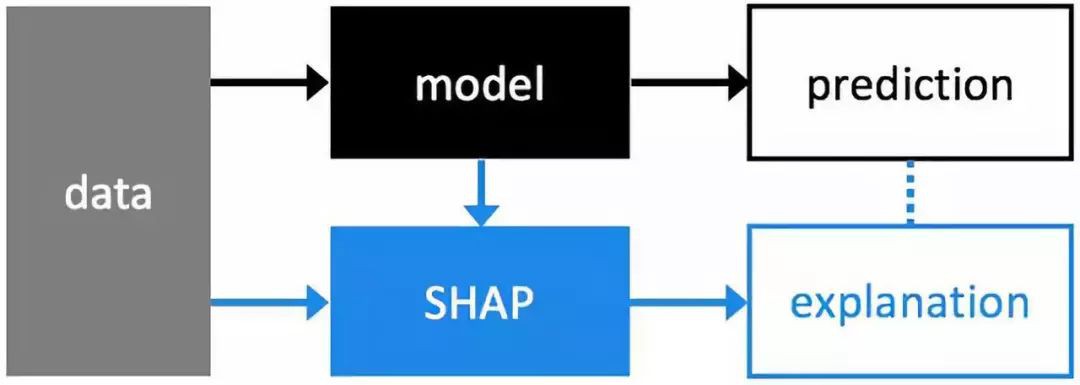
Top5 SHAP:一個解釋任何機器模型輸出的統一方法
(https://github.com/slundberg/shap)
解釋機器學習模型並不容易。然而,它對許多商業應用程式來說非常重要。幸運的是,有一些很棒的庫可以幫助我們完成這項任務。在許多應用程式中,我們需要知道、理解或證明輸入變數在模型中的運作方式,以及它們如何影響最終的模型預測。
SHAP (SHapley Additive exPlanations)是一種解釋任何機器學習模型輸出的統一方法。SHAP將博弈論與區域性解釋聯絡起來,並結合了之前的幾種方法。
安裝
SHAP可以從PyPI安裝
pip install shap
或conda -forge
conda install -c conda-forge shap
用法
有很多不同的模型和方法可以使用這個包。在這裡,我將以DeepExplainer中的一個例子為例。
Deep SHAP是深度學習模型中SHAP值的一種高速近似演演算法,它基於與DeepLIFT的連線,如SHAP的NIPS論文所述(https://arxiv.org/abs/1802.03888)。
下麵這個例子可以看到SHAP如何被用來解釋MNIST資料集的Keras模型結果:
# this is the code from https://github.com/keras-team/keras/blob/master/examples/mnist_cnn.py
from __future__ import print_function
import keras
from keras.datasets import mnist
from keras.models import Sequential
from keras.layers import Dense, Dropout, Flatten
from keras.layers import Conv2D, MaxPooling2D
from keras import backend as K
batch_size = 128
num_classes = 10
epochs = 12
# input image dimensions
img_rows, img_cols = 28, 28
# the data, split between train and test sets
(x_train, y_train), (x_test, y_test) = mnist.load_data()
if K.image_data_format() == 'channels_first':
 x_train = x_train.reshape(x_train.shape[0], 1, img_rows, img_cols)
 x_test = x_test.reshape(x_test.shape[0], 1, img_rows, img_cols)
 input_shape = (1, img_rows, img_cols)
else:
 x_train = x_train.reshape(x_train.shape[0], img_rows, img_cols, 1)
 x_test = x_test.reshape(x_test.shape[0], img_rows, img_cols, 1)
 input_shape = (img_rows, img_cols, 1)
x_train = x_train.astype('float32')
x_test = x_test.astype('float32')
x_train /= 255
x_test /= 255
print('x_train shape:', x_train.shape)
print(x_train.shape[0], 'train samples')
print(x_test.shape[0], 'test samples')
# convert class vectors to binary class matrices
y_train = keras.utils.to_categorical(y_train, num_classes)
y_test = keras.utils.to_categorical(y_test, num_classes)
model = Sequential()
model.add(Conv2D(32, kernel_size=(3, 3),
 activation='relu',
 input_shape=input_shape))
model.add(Conv2D(64, (3, 3), activation='relu'))
model.add(MaxPooling2D(pool_size=(2, 2)))
model.add(Dropout(0.25))
model.add(Flatten())
model.add(Dense(128, activation='relu'))
model.add(Dropout(0.5))
model.add(Dense(num_classes, activation='softmax'))
model.compile(loss=keras.losses.categorical_crossentropy,
 optimizer=keras.optimizers.Adadelta(),
 metrics=['accuracy'])
model.fit(x_train, y_train,
 batch_size=batch_size,
 epochs=epochs,
 verbose=1,
 validation_data=(x_test, y_test))
score = model.evaluate(x_test, y_test, verbose=0)
print('Test loss:', score[0])
print('Test accuracy:', score[1])
(左右滑動可檢視完整程式碼)
Top4 Optimus:實現敏捷資料科學工作流

(https://github.com/ironmussa/Optimus)
Optimus V2旨在讓資料清理更容易。這個API的設計對新手來說超級簡單,對使用pandas的人來說也非常熟悉。Optimus擴充套件了Spark DataFrame功能,添加了.rows和.cols屬性。
使用Optimus,你可以以分散式的方式清理資料、準備資料、分析資料、建立分析器和圖表,並執行機器學習和深度學習,因為它的後端有Spark、TensorFlow和Keras。
Optimus是資料科學敏捷方法的完美工具,因為它幾乎可以幫助你完成整個過程的所有步驟,並且可以輕鬆地連線到其他庫和工具。
安裝
pip install optimuspyspark
用法
在這個示例中,你可以從 URL 載入資料,對其進行轉換,並應用一些預定義的清理功能:
from optimus import Optimus
op = Optimus()
# This is a custom function
def func(value, arg):
 return "this was a number"
df =op.load.url("https://raw.githubusercontent.com/ironmussa/Optimus/master/examples/foo.csv")
df
 .rows.sort("product","desc")
 .cols.lower(["firstName","lastName"])
 .cols.date_transform("birth", "new_date", "yyyy/MM/dd", "dd-MM-YYYY")
 .cols.years_between("birth", "years_between", "yyyy/MM/dd")
 .cols.remove_accents("lastName")
 .cols.remove_special_chars("lastName")
 .cols.replace("product","taaaccoo","taco")
 .cols.replace("product",["piza","pizzza"],"pizza")
 .rows.drop(df["id"]<7)
 .cols.drop("dummyCol")
 .cols.rename(str.lower)
 .cols.apply_by_dtypes("product",func,"string", data_type="integer")
 .cols.trim("*")
 .show()
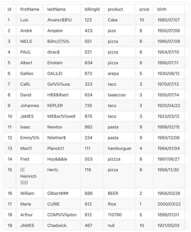
你可以將這個表格
轉換為這樣:
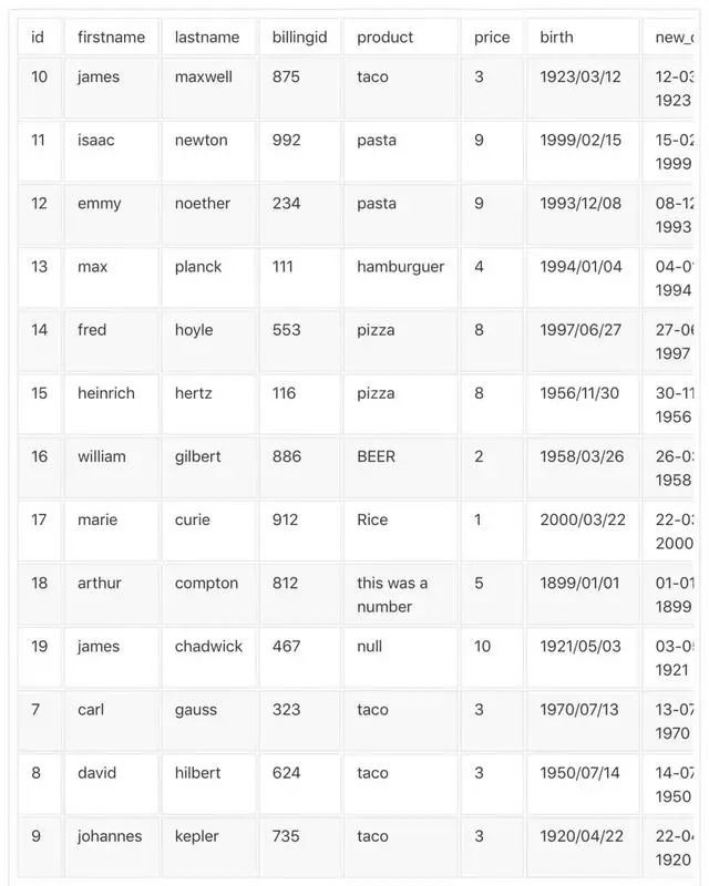
是不是很酷?
Top4 spacy:工業級自然語言處理

spaCy旨在幫助你完成實際的工作——構建真實的產品,或收集真實的見解。這個庫尊重你的時間,儘量避免浪費。它易於安裝,而且它的API簡單而高效。spaCy被視為自然語言處理的Ruby on Rails。 spaCy是為深度學習準備文字的最佳方法。它與TensorFlow、PyTorch、Scikit-learn、Gensim以及Python強大的AI生態系統的其他部分無縫互動。使用spaCy,你可以很容易地為各種NLP問題構建語言複雜的統計模型。 下麵是主頁面的一個示例: 在這個示例中,我們首先下載English tokenizer, tagger, parser, NER和word vectors。然後建立一些文字,列印找到的物體、短語和概念,最後確定兩個短語的語意相似性。執行這段程式碼,你會得到: Top2 jupytext安裝
pip3 install spacy
$ python3 -m spacy download en
# python -m spacy download en_core_web_sm
import spacy
# Load English tokenizer, tagger, parser, NER and word vectors
nlp = spacy.load('en_core_web_sm')
# Process whole documents
text = (u"When Sebastian Thrun started working on self-driving cars at "
 u"Google in 2007, few people outside of the company took him "
 u"seriously. “I can tell you very senior CEOs of major American "
 u"car companies would shake my hand and turn away because I wasn’t "
 u"worth talking to,” said Thrun, now the co-founder and CEO of "
 u"online higher education startup Udacity, in an interview with "
 u"Recode earlier this week.")
doc = nlp(text)
# Find named entities, phrases and concepts
for entity in doc.ents:
 print(entity.text, entity.label_)
# Determine semantic similarities
doc1 = nlp(u"my fries were super gross")
doc2 = nlp(u"such disgusting fries")
similarity = doc1.similarity(doc2)
print(doc1.text, doc2.text, similarity)
Sebastian Thrun PERSON
Google ORG
2007 DATE
American NORP
Thrun PERSON
Recode ORG
earlier this week DATE
my fries were super gross such disgusting fries 0.7139701635071919

(https://mybinder.org)
對我來說,jupytext是年度最佳。幾乎所有人都在像Jupyter這樣的筆記本上工作,但是我們也在專案的更核心部分使用像PyCharm這樣的IDE。
好訊息是,你可以在自己喜歡的IDE中起草和測試普通指令碼,在使用Jupytext時可以將IDE作為notebook在Jupyter中開啟。在Jupyter中執行notebook以生成輸出,關聯.ipynb表示,並作為普通指令碼或傳統Jupyter notebook 進行儲存和分享。
下圖展示了這個包的作用:
pip install jupytext --upgrade
然後,配置Jupyter使用Jupytext:
使用jupyter notebook –generate-config生成Jupyter配置
編輯.jupyter/jupyter_notebook_config.py,並附加以下程式碼:
c.NotebookApp.contents_manager_class = "jupytext.TextFileContentsManager"
重啟Jupyter,即執行:
jupyter notebook
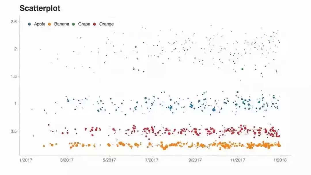
Top1 Chartify:建立圖表的Python庫
(https://xkcd.com/1945/)
Chartify是Python的年度最佳庫。
在Python世界中建立一個像樣的圖很費時間。幸運的是,我們有像Seaborn之類的庫,但問題是他們的plots不是動態的。
然後就出現了Bokeh——這是一個超棒的庫,但用它來創造互動情節仍很痛苦。
Chartify建立在Bokeh之上,但它簡單得多。
Chartify的特性:
- 一致的輸入資料格式:轉換資料所需的時間更少。所有繪圖函式都使用一致、整潔的輸入資料格式。
- 智慧預設樣式:建立漂亮的圖表,幾乎不需要自定義。
- 簡單API:API盡可能直觀和容易學習。
- 靈活性:Chartify是建立在Bokeh之上的,所以如果你需要更多的控制,你可以使用Bokeh的API。
安裝
Chartify可以透過pip安裝:
pip3 install chartify
用法
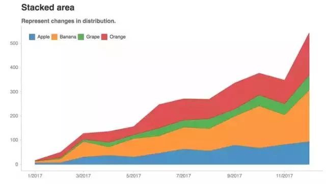
假設我們想要建立這個圖表:
import pandas as pd
import chartify
# Generate example data
data = chartify.examples.example_data()
total_quantity_by_month_and_fruit = (data.groupby(
 [data['date'] + pd.offsets.MonthBegin(-1), 'fruit'])['quantity'].sum()
 .reset_index().rename(columns={'date': 'month'})
 .sort_values('month'))
print(total_quantity_by_month_and_fruit.head())
month fruit quantity
0 2017-01-01 Apple 7
1 2017-01-01 Banana 6
2 2017-01-01 Grape 1
3 2017-01-01 Orange 2
4 2017-02-01 Apple 8
現在我們可以把它畫出來:
# Plot the data
ch = chartify.Chart(blank_labels=True, x_axis_type='datetime')
ch.set_title("Stacked area")
ch.set_subtitle("Represent changes in distribution.")
ch.plot.area(
 data_frame=total_quantity_by_month_and_fruit,
 x_column='month',
 y_column='quantity',
 color_column='fruit',
 stacked=True)
ch.show('png')
超級容易建立一個互動的plot。
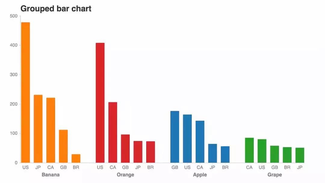
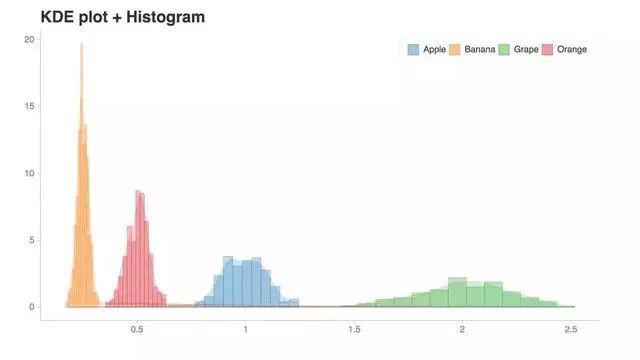
更多示例: