作者： Shivam Bansal 翻譯：申利彬校對：丁楠雅

本文約2300字，建議閱讀8分鐘。

本文將詳細介紹文字分類問題並用Python實現這個過程。

引言

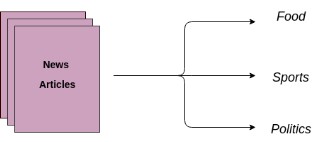
文字分類是商業問題中常見的自然語言處理任務，標的是自動將文字檔案分到一個或多個已定義好的類別中。文字分類的一些例子如下：

分析社交媒體中的大眾情感
鑒別垃圾郵件和非垃圾郵件
自動標註客戶問詢
將新聞文章按主題分類

本文將詳細介紹文字分類問題並用Python實現這個過程：

文字分類是有監督學習的一個例子，它使用包含文字檔案和標簽的資料集來訓練一個分類器。端到端的文字分類訓練主要由三個部分組成：

1. 準備資料集：第一步是準備資料集，包括載入資料集和執行基本預處理，然後把資料集分為訓練集和驗證集。

特徵工程：第二步是特徵工程，將原始資料集被轉換為用於訓練機器學習模型的平坦特徵（flat features），並從現有資料特徵建立新的特徵。

2. 模型訓練：最後一步是建模，利用標註資料集訓練機器學習模型。

3. 進一步提高分類器效能：本文還將討論用不同的方法來提高文字分類器的效能。

註意：本文不深入講述NLP任務，如果你想先複習下基礎知識，可以透過這篇文章

https://www.analyticsvidhya.com/blog/2017/01/ultimate-guide-to-understand-implement-natural-language-processing-codes-in-python/

準備好你的機器

先安裝基本元件，建立Python的文字分類框架。首先匯入所有所需的庫。如果你沒有安裝這些庫，可以透過以下官方連結來安裝它們。

Pandas:https://pandas.pydata.org/pandas-docs/stable/install.html
Scikit-learn:http://scikit-learn.org/stable/install.html
XGBoost:http://xgboost.readthedocs.io/en/latest/build.html
TextBlob:http://textblob.readthedocs.io/en/dev/install.html
Keras:https://keras.io/#installation

#匯入資料集預處理、特徵工程和模型訓練所需的庫

from sklearn import model_selection, preprocessing, linear_model, naive_bayes, metrics, svm

from sklearn.feature_extraction.text import TfidfVectorizer, CountVectorizer

from sklearn import decomposition, ensemble

import pandas, xgboost, numpy, textblob, string

from keras.preprocessing import text, sequence

from keras import layers, models, optimizers

一、準備資料集

在本文中，我使用亞馬遜的評論資料集，它可以從這個連結下載：

https://gist.github.com/kunalj101/ad1d9c58d338e20d09ff26bcc06c4235

這個資料集包含3.6M的文字評論內容及其標簽，我們只使用其中一小部分資料。首先，將下載的資料載入到包含兩個列（文字和標簽）的pandas的資料結構（dataframe）中。

資料集連結：

https://drive.google.com/drive/folders/0Bz8a_Dbh9Qhbfll6bVpmNUtUcFdjYmF2SEpmZUZUcVNiMUw1TWN6RDV3a0JHT3kxLVhVR2M

#載入資料集

data = open(‘data/corpus’).read()

labels, texts = [], []

for i, line in enumerate(data.split(“\n”)):

content = line.split()

labels.append(content[0])

texts.append(content[1])

#建立一個dataframe，列名為text和label

trainDF = pandas.DataFrame()

trainDF[‘text’] = texts

trainDF[‘label’] = labels

接下來，我們將資料集分為訓練集和驗證集，這樣我們可以訓練和測試分類器。另外，我們將編碼我們的標的列，以便它可以在機器學習模型中使用:

#將資料集分為訓練集和驗證集

train_x, valid_x, train_y, valid_y = model_selection.train_test_split(trainDF[‘text’], trainDF[‘label’])

# label編碼為標的變數

encoder = preprocessing.LabelEncoder()

train_y = encoder.fit_transform(train_y)

valid_y = encoder.fit_transform(valid_y)

二、特徵工程

接下來是特徵工程，在這一步，原始資料將被轉換為特徵向量，另外也會根據現有的資料建立新的特徵。為了從資料集中選出重要的特徵，有以下幾種方式：

計數向量作為特徵
TF-IDF向量作為特徵

單個詞語級別
多個詞語級別（N-Gram）
詞性級別

詞嵌入作為特徵
基於文字/NLP的特徵
主題模型作為特徵

接下來分別看看它們如何實現：

2.1 計數向量作為特徵

計數向量是資料集的矩陣表示，其中每行代表來自語料庫的檔案，每串列示來自語料庫的術語，並且每個單元格表示特定檔案中特定術語的頻率計數：

#建立一個向量計數器物件

count_vect = CountVectorizer(analyzer=’word’, token_pattern=r’\w{1,}’)

count_vect.fit(trainDF[‘text’])

#使用向量計數器物件轉換訓練集和驗證集

xtrain_count = count_vect.transform(train_x)

xvalid_count = count_vect.transform(valid_x)

2.2 TF-IDF向量作為特徵

TF-IDF的分數代表了詞語在檔案和整個語料庫中的相對重要性。TF-IDF分數由兩部分組成：第一部分是計算標準的詞語頻率（TF），第二部分是逆檔案頻率（IDF）。其中計算語料庫中檔案總數除以含有該詞語的檔案數量，然後再取對數就是逆檔案頻率。

TF(t)=（該詞語在檔案出現的次數）/（檔案中詞語的總數）

IDF(t)= log_e（檔案總數/出現該詞語的檔案總數）

TF-IDF向量可以由不同級別的分詞產生（單個詞語，詞性，多個詞（n-grams））

詞語級別TF-IDF：矩陣代表了每個詞語在不同檔案中的TF-IDF分數。
N-gram級別TF-IDF: N-grams是多個詞語在一起的組合，這個矩陣代表了N-grams的TF-IDF分數。
詞性級別TF-IDF：矩陣代表了語料中多個詞性的TF-IDF分數。

#詞語級tf-idf

tfidf_vect = TfidfVectorizer(analyzer=’word’, token_pattern=r’\w{1,}’, max_features=5000)

tfidf_vect.fit(trainDF[‘text’])

xtrain_tfidf = tfidf_vect.transform(train_x)

xvalid_tfidf = tfidf_vect.transform(valid_x)

# ngram 級tf-idf

tfidf_vect_ngram = TfidfVectorizer(analyzer=’word’, token_pattern=r’\w{1,}’, ngram_range=(2,3), max_features=5000)

tfidf_vect_ngram.fit(trainDF[‘text’])

xtrain_tfidf_ngram = tfidf_vect_ngram.transform(train_x)

xvalid_tfidf_ngram = tfidf_vect_ngram.transform(valid_x)

#詞性級tf-idf

tfidf_vect_ngram_chars = TfidfVectorizer(analyzer=’char’, token_pattern=r’\w{1,}’, ngram_range=(2,3), max_features=5000)

tfidf_vect_ngram_chars.fit(trainDF[‘text’])

xtrain_tfidf_ngram_chars = tfidf_vect_ngram_chars.transform(train_x)

xvalid_tfidf_ngram_chars = tfidf_vect_ngram_chars.transform(valid_x)

2.3 詞嵌入

詞嵌入是使用稠密向量代表詞語和檔案的一種形式。向量空間中單詞的位置是從該單詞在文字中的背景關係學習到的，詞嵌入可以使用輸入語料本身訓練，也可以使用預先訓練好的詞嵌入模型生成，詞嵌入模型有：Glove, FastText,Word2Vec。它們都可以下載，並用遷移學習的方式使用。想瞭解更多的詞嵌入資料，可以訪問：

https://www.analyticsvidhya.com/blog/2017/06/word-embeddings-count-word2veec/

接下來介紹如何在模型中使用預先訓練好的詞嵌入模型，主要有四步：

1. 載入預先訓練好的詞嵌入模型

2. 建立一個分詞物件

3. 將文字檔案轉換為分詞序列並填充它們

4. 建立分詞和各自嵌入的對映

#載入預先訓練好的詞嵌入向量

embeddings_index = {}

for i, line in enumerate(open(‘data/wiki-news-300d-1M.vec’)):

values = line.split()

embeddings_index[values[0]] = numpy.asarray(values[1:], dtype=’float32′)

#建立一個分詞器

token = text.Tokenizer()

token.fit_on_texts(trainDF[‘text’])

word_index = token.word_index

#將文字轉換為分詞序列，並填充它們保證得到相同長度的向量

train_seq_x = sequence.pad_sequences(token.texts_to_sequences(train_x), maxlen=70)

valid_seq_x = sequence.pad_sequences(token.texts_to_sequences(valid_x), maxlen=70)

#建立分詞嵌入對映

embedding_matrix = numpy.zeros((len(word_index) + 1, 300))

for word, i in word_index.items():

embedding_vector = embeddings_index.get(word)

if embedding_vector is not None:

embedding_matrix[i] = embedding_vector

2.4 基於文字/NLP的特徵

建立許多額外基於文字的特徵有時可以提升模型效果。比如下麵的例子：

檔案的詞語計數—檔案中詞語的總數量
檔案的詞性計數—檔案中詞性的總數量
檔案的平均字密度–檔案中使用的單詞的平均長度
完整文章中的標點符號出現次數–檔案中標點符號的總數量
整篇文章中的大寫次數—檔案中大寫單詞的數量
完整文章中標題出現的次數—檔案中適當的主題（標題）的總數量
詞性標註的頻率分佈

名詞數量
動詞數量
形容詞數量
副詞數量
代詞數量

這些特徵有很強的實驗性質，應該具體問題具體分析。

trainDF[‘char_count’] = trainDF[‘text’].apply(len)

trainDF[‘word_count’] = trainDF[‘text’].apply(lambda x: len(x.split()))

trainDF[‘word_density’] = trainDF[‘char_count’] / (trainDF[‘word_count’]+1)

trainDF[‘punctuation_count’] = trainDF[‘text’].apply(lambda x: len(“”.join(_ for _ in x if _ in string.punctuation)))

trainDF[‘title_word_count’] = trainDF[‘text’].apply(lambda x: len([wrd for wrd in x.split() if wrd.istitle()]))

trainDF[‘upper_case_word_count’] = trainDF[‘text’].apply(lambda x: len([wrd for wrd in x.split() if wrd.isupper()]))

trainDF[‘char_count’] = trainDF[‘text’].apply(len)

trainDF[‘word_count’] = trainDF[‘text’].apply(lambda x: len(x.split()))

trainDF[‘word_density’] = trainDF[‘char_count’] / (trainDF[‘word_count’]+1)

trainDF[‘punctuation_count’] = trainDF[‘text’].apply(lambda x: len(“”.join(_ for _ in x if _ in string.punctuation)))

trainDF[‘title_word_count’] = trainDF[‘text’].apply(lambda x: len([wrd for wrd in x.split() if wrd.istitle()]))

trainDF[‘upper_case_word_count’] = trainDF[‘text’].apply(lambda x: len([wrd for wrd in x.split() if wrd.isupper()]))

pos_family = {

‘noun’ : [‘NN’,’NNS’,’NNP’,’NNPS’],

‘pron’ : [‘PRP’,’PRP$’,’WP’,’WP$’],

‘verb’ : [‘VB’,’VBD’,’VBG’,’VBN’,’VBP’,’VBZ’],

‘adj’ : [‘JJ’,’JJR’,’JJS’],

‘adv’ : [‘RB’,’RBR’,’RBS’,’WRB’]

}

#檢查和獲得特定句子中的單詞的詞性標簽數量

def check_pos_tag(x, flag):

cnt = 0

try:

wiki = textblob.TextBlob(x)

for tup in wiki.tags:

ppo = list(tup)[1]

if ppo in pos_family[flag]:

cnt += 1

except:

pass

return cnt

trainDF[‘noun_count’] = trainDF[‘text’].apply(lambda x: check_pos_tag(x, ‘noun’))

trainDF[‘verb_count’] = trainDF[‘text’].apply(lambda x: check_pos_tag(x, ‘verb’))

trainDF[‘adj_count’] = trainDF[‘text’].apply(lambda x: check_pos_tag(x, ‘adj’))

trainDF[‘adv_count’] = trainDF[‘text’].apply(lambda x: check_pos_tag(x, ‘adv’))

trainDF[‘pron_count’] = trainDF[‘text’].apply(lambda x: check_pos_tag(x, ‘pron’))

2.5 主題模型作為特徵

主題模型是從包含重要資訊的檔案集中識別片語（主題）的技術，我已經使用LDA生成主題模型特徵。LDA是一個從固定數量的主題開始的迭代模型，每一個主題代表了詞語的分佈，每一個檔案表示了主題的分佈。雖然分詞本身沒有意義，但是由主題表達出的詞語的機率分佈可以傳達檔案思想。如果想瞭解更多主題模型，請訪問：

https://www.analyticsvidhya.com/blog/2016/08/beginners-guide-to-topic-modeling-in-python/

我們看看主題模型執行過程：

#訓練主題模型

lda_model = decomposition.LatentDirichletAllocation(n_components=20, learning_method=’online’, max_iter=20)

X_topics = lda_model.fit_transform(xtrain_count)

topic_word = lda_model.components_

vocab = count_vect.get_feature_names()

#視覺化主題模型

n_top_words = 10

topic_summaries = []

for i, topic_dist in enumerate(topic_word):

topic_words = numpy.array(vocab)[numpy.argsort(topic_dist)][:-(n_top_words+1):-1]

topic_summaries.append(‘ ‘.join(topic_words)

三、建模

文字分類框架的最後一步是利用之前建立的特徵訓練一個分類器。關於這個最終的模型，機器學習中有很多模型可供選擇。我們將使用下麵不同的分類器來做文字分類：

樸素貝葉斯分類器
線性分類器
支援向量機（SVM）
Bagging Models
Boosting Models
淺層神經網路
深層神經網路

摺積神經網路（CNN）
LSTM
GRU
雙向RNN
迴圈摺積神經網路（RCNN）
其它深層神經網路的變種

接下來我們詳細介紹並使用這些模型。下麵的函式是訓練模型的通用函式，它的輸入是分類器、訓練資料的特徵向量、訓練資料的標簽，驗證資料的特徵向量。我們使用這些輸入訓練一個模型，並計算準確度。

def train_model(classifier, feature_vector_train, label, feature_vector_valid, is_neural_net=False):

# fit the training dataset on the classifier

classifier.fit(feature_vector_train, label)

# predict the labels on validation dataset

predictions = classifier.predict(feature_vector_valid)

if is_neural_net:

predictions = predictions.argmax(axis=-1)

return metrics.accuracy_score(predictions, valid_y)

3.1 樸素貝葉斯

利用sklearn框架，在不同的特徵下實現樸素貝葉斯模型。

樸素貝葉斯是一種基於貝葉斯定理的分類技術，並且假設預測變數是獨立的。樸素貝葉斯分類器假設一個類別中的特定特徵與其它存在的特徵沒有任何關係。

想瞭解樸素貝葉斯演演算法細節可點選：

A Naive Bayes classifier assumes that the presence of a particular feature in a class is unrelated to the presence of any other feature

#特徵為計數向量的樸素貝葉斯

accuracy = train_model(naive_bayes.MultinomialNB(), xtrain_count, train_y, xvalid_count)

print “NB, Count Vectors: “, accuracy

#特徵為詞語級別TF-IDF向量的樸素貝葉斯

accuracy = train_model(naive_bayes.MultinomialNB(), xtrain_tfidf, train_y, xvalid_tfidf)

print “NB, WordLevel TF-IDF: “, accuracy

#特徵為多個詞語級別TF-IDF向量的樸素貝葉斯

accuracy = train_model(naive_bayes.MultinomialNB(), xtrain_tfidf_ngram, train_y, xvalid_tfidf_ngram)

print “NB, N-Gram Vectors: “, accuracy

#特徵為詞性級別TF-IDF向量的樸素貝葉斯

accuracy = train_model(naive_bayes.MultinomialNB(), xtrain_tfidf_ngram_chars, train_y, xvalid_tfidf_ngram_chars)

print “NB, CharLevel Vectors: “, accuracy

#輸出結果

NB, Count Vectors: 0.7004

NB, WordLevel TF-IDF: 0.7024

NB, N-Gram Vectors: 0.5344

NB, CharLevel Vectors: 0.6872

3.2 線性分類器

實現一個線性分類器（Logistic Regression）：Logistic回歸透過使用logistic / sigmoid函式估計機率來度量類別因變數與一個或多個獨立變數之間的關係。如果想瞭解更多關於logistic回歸，請訪問：

https://www.analyticsvidhya.com/blog/2015/10/basics-logistic-regression/

# Linear Classifier on Count Vectors

accuracy = train_model(linear_model.LogisticRegression(), xtrain_count, train_y, xvalid_count)

print “LR, Count Vectors: “, accuracy

#特徵為詞語級別TF-IDF向量的線性分類器

accuracy = train_model(linear_model.LogisticRegression(), xtrain_tfidf, train_y, xvalid_tfidf)

print “LR, WordLevel TF-IDF: “, accuracy

#特徵為多個詞語級別TF-IDF向量的線性分類器

accuracy = train_model(linear_model.LogisticRegression(), xtrain_tfidf_ngram, train_y, xvalid_tfidf_ngram)

print “LR, N-Gram Vectors: “, accuracy

#特徵為詞性級別TF-IDF向量的線性分類器

accuracy = train_model(linear_model.LogisticRegression(), xtrain_tfidf_ngram_chars, train_y, xvalid_tfidf_ngram_chars)

print “LR, CharLevel Vectors: “, accuracy

#輸出結果

LR, Count Vectors: 0.7048

LR, WordLevel TF-IDF: 0.7056

LR, N-Gram Vectors: 0.4896

LR, CharLevel Vectors: 0.7012

3.3 實現支援向量機模型

支援向量機（SVM）是監督學習演演算法的一種，它可以用來做分類或回歸。該模型提取了分離兩個類的最佳超平面或線。如果想瞭解更多關於SVM，請訪問：

https://www.analyticsvidhya.com/blog/2017/09/understaing-support-vector-machine-example-code/

#特徵為多個詞語級別TF-IDF向量的SVM

accuracy = train_model(svm.SVC(), xtrain_tfidf_ngram, train_y, xvalid_tfidf_ngram)

print “SVM, N-Gram Vectors: “, accuracy

#輸出結果

SVM, N-Gram Vectors: 0.5296

3.4 Bagging Model

實現一個隨機森林模型：隨機森林是一種整合模型，更準確地說是Bagging model。它是基於樹模型家族的一部分。如果想瞭解更多關於隨機森林，請訪問：

https://www.analyticsvidhya.com/blog/2014/06/introduction-random-forest-simplified/

#特徵為計數向量的RF

accuracy = train_model(ensemble.RandomForestClassifier(), xtrain_count, train_y, xvalid_count)

print “RF, Count Vectors: “, accuracy

#特徵為詞語級別TF-IDF向量的RF

accuracy = train_model(ensemble.RandomForestClassifier(), xtrain_tfidf, train_y, xvalid_tfidf)

print “RF, WordLevel TF-IDF: “, accuracy

#輸出結果

RF, Count Vectors: 0.6972

RF, WordLevel TF-IDF: 0.6988

3.5 Boosting Model

實現一個Xgboost模型：Boosting model是另外一種基於樹的整合模型。Boosting是一種機器學習整合元演演算法，主要用於減少模型的偏差，它是一組機器學習演演算法，可以把弱學習器提升為強學習器。其中弱學習器指的是與真實類別隻有輕微相關的分類器（比隨機猜測要好一點）。如果想瞭解更多，請訪問：

https://www.analyticsvidhya.com/blog/2016/01/xgboost-algorithm-easy-steps/

#特徵為計數向量的Xgboost

accuracy = train_model(xgboost.XGBClassifier(), xtrain_count.tocsc(), train_y, xvalid_count.tocsc())

print “Xgb, Count Vectors: “, accuracy

#特徵為詞語級別TF-IDF向量的Xgboost

accuracy = train_model(xgboost.XGBClassifier(), xtrain_tfidf.tocsc(), train_y, xvalid_tfidf.tocsc())

print “Xgb, WordLevel TF-IDF: “, accuracy

#特徵為詞性級別TF-IDF向量的Xgboost

accuracy = train_model(xgboost.XGBClassifier(), xtrain_tfidf_ngram_chars.tocsc(), train_y, xvalid_tfidf_ngram_chars.tocsc())

print “Xgb, CharLevel Vectors: “, accuracy

#輸出結果

Xgb, Count Vectors: 0.6324

Xgb, WordLevel TF-IDF: 0.6364

Xgb, CharLevel Vectors: 0.6548

3.6 淺層神經網路

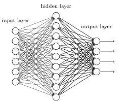
神經網路被設計成與生物神經元和神經系統類似的數學模型，這些模型用於發現被標註資料中存在的複雜樣式和關係。一個淺層神經網路主要包含三層神經元-輸入層、隱藏層、輸出層。如果想瞭解更多關於淺層神經網路，請訪問：

https://www.analyticsvidhya.com/blog/2017/05/neural-network-from-scratch-in-python-and-r/

def create_model_architecture(input_size):

# create input layer

input_layer = layers.Input((input_size, ), sparse=True)

# create hidden layer

hidden_layer = layers.Dense(100, activation=”relu”)(input_layer)

# create output layer

output_layer = layers.Dense(1, activation=”sigmoid”)(hidden_layer)

classifier = models.Model(inputs = input_layer, outputs = output_layer)

classifier.compile(optimizer=optimizers.Adam(), loss=’binary_crossentropy’)

return classifier

classifier = create_model_architecture(xtrain_tfidf_ngram.shape[1])

accuracy = train_model(classifier, xtrain_tfidf_ngram, train_y, xvalid_tfidf_ngram, is_neural_net=True)

print “NN, Ngram Level TF IDF Vectors”, accuracy

#輸出結果：

Epoch 1/1

7500/7500 [==============================] – 1s 67us/step – loss: 0.6909

NN, Ngram Level TF IDF Vectors 0.5296

3.7 深層神經網路

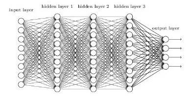
深層神經網路是更複雜的神經網路，其中隱藏層執行比簡單Sigmoid或Relu啟用函式更複雜的操作。不同型別的深層學習模型都可以應用於文字分類問題。

摺積神經網路

摺積神經網路中，輸入層上的摺積用來計算輸出。本地連線結果中，每一個輸入單元都會連線到輸出神經元上。每一層網路都應用不同的濾波器（filter）並組合它們的結果。

如果想瞭解更多關於摺積神經網路，請訪問：

https://www.analyticsvidhya.com/blog/2017/06/architecture-of-convolutional-neural-networks-simplified-demystified/

def create_cnn():

# Add an Input Layer

input_layer = layers.Input((70, ))

# Add the word embedding Layer

embedding_layer = layers.Embedding(len(word_index) + 1, 300, weights=[embedding_matrix], trainable=False)(input_layer)

embedding_layer = layers.SpatialDropout1D(0.3)(embedding_layer)

# Add the convolutional Layer

conv_layer = layers.Convolution1D(100, 3, activation=”relu”)(embedding_layer)

# Add the pooling Layer

pooling_layer = layers.GlobalMaxPool1D()(conv_layer)

# Add the output Layers

output_layer1 = layers.Dense(50, activation=”relu”)(pooling_layer)

output_layer1 = layers.Dropout(0.25)(output_layer1)

output_layer2 = layers.Dense(1, activation=”sigmoid”)(output_layer1)

# Compile the model

model = models.Model(inputs=input_layer, outputs=output_layer2)

model.compile(optimizer=optimizers.Adam(), loss=’binary_crossentropy’)

return model

classifier = create_cnn()

accuracy = train_model(classifier, train_seq_x, train_y, valid_seq_x, is_neural_net=True)

print “CNN, Word Embeddings”, accuracy

#輸出結果

Epoch 1/1

7500/7500 [==============================] – 12s 2ms/step – loss: 0.5847

CNN, Word Embeddings 0.5296

迴圈神經網路-LSTM

與前饋神經網路不同，前饋神經網路的啟用輸出僅在一個方向上傳播，而迴圈神經網路的啟用輸出在兩個方向傳播（從輸入到輸出，從輸出到輸入）。因此在神經網路架構中產生迴圈，充當神經元的“記憶狀態”，這種狀態使神經元能夠記住迄今為止學到的東西。RNN中的記憶狀態優於傳統的神經網路，但是被稱為梯度彌散的問題也因這種架構而產生。這個問題導致當網路有很多層的時候，很難學習和調整前面網路層的引數。為瞭解決這個問題，開發了稱為LSTM（Long Short Term Memory）模型的新型RNN：

如果想瞭解更多關於LSTM，請訪問：

https://www.analyticsvidhya.com/blog/2017/12/fundamentals-of-deep-learning-introduction-to-lstm/

def create_rnn_lstm():

# Add an Input Layer

input_layer = layers.Input((70, ))

# Add the word embedding Layer

embedding_layer = layers.Embedding(len(word_index) + 1, 300, weights=[embedding_matrix], trainable=False)(input_layer)

embedding_layer = layers.SpatialDropout1D(0.3)(embedding_layer)

# Add the LSTM Layer

lstm_layer = layers.LSTM(100)(embedding_layer)

# Add the output Layers

output_layer1 = layers.Dense(50, activation=”relu”)(lstm_layer)

output_layer1 = layers.Dropout(0.25)(output_layer1)

output_layer2 = layers.Dense(1, activation=”sigmoid”)(output_layer1)

# Compile the model

model = models.Model(inputs=input_layer, outputs=output_layer2)

model.compile(optimizer=optimizers.Adam(), loss=’binary_crossentropy’)

return model

classifier = create_rnn_lstm()

accuracy = train_model(classifier, train_seq_x, train_y, valid_seq_x, is_neural_net=True)

print “RNN-LSTM, Word Embeddings”, accuracy

#輸出結果

Epoch 1/1

7500/7500 [==============================] – 22s 3ms/step – loss: 0.6899

RNN-LSTM, Word Embeddings 0.5124

迴圈神經網路-GRU

門控遞迴單元是另一種形式的遞迴神經網路,我們在網路中新增一個GRU層來代替LSTM。

defcreate_rnn_gru():

# Add an Input Layer

input_layer = layers.Input((70, ))

# Add the word embedding Layer

embedding_layer = layers.Embedding(len(word_index) + 1, 300, weights=[embedding_matrix], trainable=False)(input_layer)

embedding_layer = layers.SpatialDropout1D(0.3)(embedding_layer)

# Add the GRU Layer

lstm_layer = layers.GRU(100)(embedding_layer)

# Add the output Layers

output_layer1 = layers.Dense(50, activation=”relu”)(lstm_layer)

output_layer1 = layers.Dropout(0.25)(output_layer1)

output_layer2 = layers.Dense(1, activation=”sigmoid”)(output_layer1)

# Compile the model

model = models.Model(inputs=input_layer, outputs=output_layer2)

model.compile(optimizer=optimizers.Adam(), loss=’binary_crossentropy’)

return model

classifier = create_rnn_gru()

accuracy = train_model(classifier, train_seq_x, train_y, valid_seq_x, is_neural_net=True)

print “RNN-GRU, Word Embeddings”, accuracy

#輸出結果

Epoch 1/1

7500/7500 [==============================] – 19s 3ms/step – loss: 0.6898

RNN-GRU, Word Embeddings 0.5124

雙向RNN

RNN層也可以被封裝在雙向層中，我們把GRU層封裝在雙向RNN網路中。

defcreate_bidirectional_rnn():

# Add an Input Layer

input_layer = layers.Input((70, ))

# Add the word embedding Layer

embedding_layer = layers.Embedding(len(word_index) + 1, 300, weights=[embedding_matrix], trainable=False)(input_layer)

embedding_layer = layers.SpatialDropout1D(0.3)(embedding_layer)

# Add the LSTM Layer

lstm_layer = layers.Bidirectional(layers.GRU(100))(embedding_layer)

# Add the output Layers

output_layer1 = layers.Dense(50, activation=”relu”)(lstm_layer)

output_layer1 = layers.Dropout(0.25)(output_layer1)

output_layer2 = layers.Dense(1, activation=”sigmoid”)(output_layer1)

# Compile the model

model = models.Model(inputs=input_layer, outputs=output_layer2)

model.compile(optimizer=optimizers.Adam(), loss=’binary_crossentropy’)

return model

classifier = create_bidirectional_rnn()

accuracy = train_model(classifier, train_seq_x, train_y, valid_seq_x, is_neural_net=True)

print “RNN-Bidirectional, Word Embeddings”, accuracy

#輸出結果

Epoch 1/1

7500/7500 [==============================] – 32s 4ms/step – loss: 0.6889

RNN-Bidirectional, Word Embeddings 0.5124

迴圈摺積神經網路

如果基本的架構已經嘗試過，則可以嘗試這些層的不同變體，如遞迴摺積神經網路，還有其它變體，比如：

層次化註意力網路（Sequence to Sequence Models with Attention）
具有註意力機制的seq2seq（Sequence to Sequence Models with Attention）
雙向迴圈摺積神經網路
更多網路層數的CNNs和RNNs

defcreate_rcnn():

# Add an Input Layer

input_layer = layers.Input((70, ))

# Add the word embedding Layer

embedding_layer = layers.Embedding(len(word_index) + 1, 300, weights=[embedding_matrix], trainable=False)(input_layer)

embedding_layer = layers.SpatialDropout1D(0.3)(embedding_layer)

# Add the recurrent layer

rnn_layer = layers.Bidirectional(layers.GRU(50, return_sequences=True))(embedding_layer)

# Add the convolutional Layer

conv_layer = layers.Convolution1D(100, 3, activation=”relu”)(embedding_layer)

# Add the pooling Layer

pooling_layer = layers.GlobalMaxPool1D()(conv_layer)

# Add the output Layers

output_layer1 = layers.Dense(50, activation=”relu”)(pooling_layer)

output_layer1 = layers.Dropout(0.25)(output_layer1)

output_layer2 = layers.Dense(1, activation=”sigmoid”)(output_layer1)

# Compile the model

model = models.Model(inputs=input_layer, outputs=output_layer2)

model.compile(optimizer=optimizers.Adam(), loss=’binary_crossentropy’)

return model

classifier = create_rcnn()

accuracy = train_model(classifier, train_seq_x, train_y, valid_seq_x, is_neural_net=True)

print “CNN, Word Embeddings”, accuracy

#輸出結果

Epoch 1/1

7500/7500 [==============================] – 11s 1ms/step – loss: 0.6902

CNN, Word Embeddings 0.5124